If you change the coefficients of a polynomial a little bit, do you change the location of its zeros a little bit? In other words, do the roots of a polynomial depend continuously on its coefficients?

You would think so, and you’d be right. Sorta.

It’s easy to see that small change to a coefficient could result in a qualitative change, such as a double root splitting into two distinct roots close together, or a real root acquiring a small imaginary part. But it’s also possible that a small change to a coefficient could cause roots to move quite a bit.

Wilkinson’s polynomial

Wilkinson’s polynomial is a famous example that makes this all clear.

Define

w(x) = (x − 1)(x − 2)(x − 3)…(x − 20) = x²⁰ − 210x¹⁹ + …

and

W(x) = w(x) − 2⁻²³ x¹⁹

so that the difference between the two polynomials is that the coefficient of x¹⁹ in the former is −210 and in the latter the coefficient is −210.0000001192.

Surely the roots of w(x) and W(x) are close together. But they’re not!

The roots of w are clearly 1, 2, 3, …, 20. But the roots of W are substantially different. Or at least some are substantially different. About half the roots didn’t move much, but the other half moved a lot. If we order the roots by their real part, the 16th root splits into two roots, 16.7308 ± 2.81263 i.

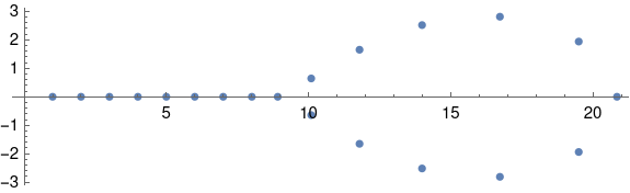
Here’s the Mathematica code that produced the plot above.

    w[x_] := Product[(x - i), {i, 1, 20}]
    W[x_] := w[x] - 2^-23 x^19
    roots = NSolve[W[x] == 0, x]
    ComplexListPlot[x /. roots]

A tiny change to one coefficient creates a change in the roots that is seven orders of magnitude larger. Wilkinson described this discovery as “traumatic.”

Modulus of continuity

The zeros of a polynomial do depend continuously on the parameters, but the modulus of continuity might be enormous.

Given some desired tolerance ε on how much the zeros are allowed to move, you can specify a corresponding degree of accuracy δ on the coefficients to meet that tolerance, but you might have to have extreme accuracy on the coefficients to have moderate accuracy on the roots. The modulus of continuity is essentially the ratio ε/δ, and this ratio might be very large. In the example above it’s roughly 8,400,000.

In terms of the δ-ε definition of continuity, for every ε there is a δ. But that δ might have to be orders of magnitude smaller than ε.

Modulus of continuity is an important concept. In applications, it might not matter that a function is continuous if the modulus of continuity is enormous. In that case the function may be discontinuous for practical purposes.

Continuity is a discrete concept—a function is either continuous or it’s not—but modulus of continuity is a continuous concept, and this distinction can resolve some apparent paradoxes.

For example, consider the sequence of functions f_n(x) = xⁿ on the interval [0, 1].  For every n, f_n is continuous, but the limit is not a continuous function: the limit equals 0 for x < 1 and equals 1 at x = 1.

But this makes sense in terms of modulus of continuity. The modulus of continuity of f_n(x) is n. So while the sequence is continuous for large n, it is becoming “less continuous” in the sense that the modulus of continuity is increasing.

The post Wilkinson’s polynomial first appeared on John D. Cook.