What is the right tool for the job?

This article is about my journey in understanding and applying Survival Models, which can be used to predict the probability of an event happening over time (e.g., recovery of a patient). I have been working as a data scientist for eight years and implementing a Survival Model for about two years. These models are underappreciated in education and industry and, therefore, unknown among most data scientists.
There are rarely resources that go beyond the fundamentals, so I want to share my experiences digging deeper into these special models. Especially when it comes to Evaluation and Dynamic Models (updating predictions over time), I came up with some solutions I have yet to see used anywhere else.
This article requires at least basic knowledge of Supervised Machine Learning Models and their application, but should also be interesting to those familiar with Survival Models to learn about or discuss challenges in real-world applications.
All code related to this post can be found here
Motivation
Many will know the feeling of facing an unknown problem for which we don’t have a solution in our toolbox yet and don’t even know whether one exists.
At a recruiting challenge, I was confronted with predicting customer churn, which I expected to be a very familiar problem. But soon, I found myself struggling with the fact that active customers of today can be the terminations of the next day. I tried to devise a solution with a classic ML model, but it didn’t feel satisfying.
I was later hired at that job and learned about the Survival approach, which considers the uncertainty of the customer status — An eureka moment for me on how to solve this and other event occurrence problems.
While recruiting other data scientists using the same challenge I saw dozens struggle with the same problem. Like myself they all came up with some solution, but it seemed like they needed to be more optimal.
While trying to find libraries and solve problems in this area, I found that there are definitely resources, but they rarely go beyond the fundamentals. It is not part of popular libraries like sklearn or fast.ai or has limited implementations like in the xgboost library
In education, there are few specialized courses on Coursera or datacamp, for example. But without this topic being mentioned in basic courses, you will probably never stumble into those. Also, the agendas of those courses feel quite shallow and outdated (e.g., only using linear models).
While they seem underappreciated in education and industry, there are many use cases where a time-to-event prediction can be useful:
- Death or recovery in medical treatment
- Failure in mechanical systems
- Customer churn
- End of strike
- End of government rule
Survival Models
Theory
The name “Survival” stems from the origins of the method in the field of medicine. While I would propose a more general term like “Time to Event Models,” “Survival Models” or “Survival Analysis” are widely accepted, so I will stick with those here.
I don’t want to talk too much about the theory but rather focus on practical applications. Two good sources for the fundamentals are this article and the lifelines library intro.
Data and Examples
I will mainly use one dataset for the notebooks and examples in this article. It is about the reign duration of political regimes (democracies and dictatorships) in 202 countries from 1946 or the year of independence to 2008.
The goal is to predict the probability of a government staying in power over time or, in other words. predict the event of a change in government. Features include mostly information about the region (e.g., continent) and government type (e.g., democracy).
Survival Targets
Good news first: In Survival Models, only the prediction targets change, while features stay the same as in classic ML models.
There are two data points of interest as targets: The event and the duration.
Event
An event can be anything from recovery in medical treatment or a customer’s churn to the end of a government rule. The target column holds the information on whether the event was observed and will be binary in most cases (there are special forms with multiple competing events, though).
If the event is not observed, it means up to a specific point, the event might occur at any later time. This uncertainty in the event information is called censoring and is the main reason why traditional regression and classification models are not the best solution.
There are different forms of censoring, but we will focus on the most common form of right-censoring here, which means that we don’t know what happens after a certain point in time.
Consider this customer churn example:

- Customer terminated contract: The event of churn has occurred
- Customer is still active: The event of churn has not occurred yet but can still occur in the future (right-censored)
- Customer left because of external circumstances (e.g., death): The event of churn has not occurred, and the customer is right-censored at the point in time when external circumstances occurred
Duration
The duration column holds the information on how long it took until the event was observed or at another specific point (e.g., date of analysis, external circumstance) in case the event is not observed yet. The duration unit depends on the data and can be anything from seconds to years.
Target Modeling
Let’s look at how we could model the targets in a Regression, Classification (if you are not familiar with those, check this), and Survival Model. The code for this section can be found here.
Modeling as a Regression Problem

A Regression Model is used to predict continuous values.
In our example, it could only use duration as a target and dismiss all information about the event. The event also cannot be used as a feature since it is unknown initially. Furthermore, the prediction will give you a number for the duration without telling you about the possibility of event occurrence.
This doesn’t seem like a good idea in most cases.
Modeling as a Classification problem

A Classification Model is used to predict discrete values and assigns probabilities to classes.
In our example, it could use an event as a target but can also incorporate fixed time durations (e.g., does the event occur after one year).
Data loss is possible since rows with no event occurrence and duration smaller than chosen fixed time duration (e.g., one year) cannot be used. You can find an example of this in the Target Modeling Notebook).
Using this method, multiple classification models can create an output close to Survival Models, but this adds a lot of complexity. For example, a monthly forecast over three years would need 36 Classification Models compared to a single Survival Model (see next section).
However, this might be a valid approach depending on the use case (e.g., we are only interested in the probability of the event occurring at a specific t) and data availability.
Modeling as a Survival Problem

Let’s see how we can overcome these disadvantages using the Survival method:
As you can see, it can include both targets as input to the model!
While Regression outputs are continuous and Classification outputs are class probabilities, the output of a Survival Model is more complicated. It can be a single continuous value that summarizes the risk of the event occurrence (hazard) and can be converted into various other measures.
More interestingly, the output can be converted to a Survival Curve with event probabilities over time. There are different ways (parameters) to turn a hazard into a Survival Curve, but most libraries can handle this for you. Neural Nets can even optimize the shape of the Survival Curve by using one output neuron for every point of the curve. These probabilities over time can be used for other metric calculations, e.g., Customer Lifetime Value.
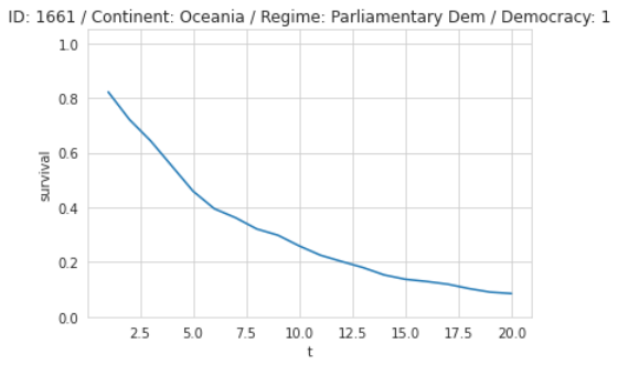
Here is a Survival Curve with probabilities for the end of government rule over the next 20 years. For example, after ten years, the probability that this democratic government from Oceania is still in power is about 23%:
Survival Approach for Survival Problems
As you can see, the Survival approach is specifically created to include event and time information and gives us very nice probabilities over time, making it the best choice for this kind of problem. There is also a really nice article with code where the author ran all three modeling approaches with actual data concluding that the Survival approach outperforms the other two.
The only exception could be a use case where we are only interested in the probability at a certain time. In this case, a classification model would also work fine.
Models and Libraries
Good News first: Survival Models adapt classic ML models like Logistic Regression, Decision Trees, and Neural Nets. Like in other areas, new developments mostly happen with Deep Learning methods.
These are the libraries I recommend when working with Survival Models:
- lifelines: Linear Models and lots of statistical functions. This is a good starting point, but most of the time will not produce the most accurate models
- pycox: Survival Models based on Neural Nets — They mainly implement loss functions that can be put on top of any pytorch architecture
- XGBSE: XGBoost implementation of Survival Models with different model complexities
You can find one Notebook for each library to see how the data needs to be prepared, and a model can be run here (02 / 03 / 04).
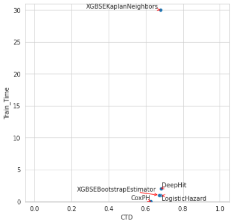
In addition, you can find a benchmark for the government data set with runtimes and quality metrics using these libraries. Here is a scatterplot from the benchmark comparing training time and Concordance (see the Evaluation section for an explanation of this metric):
I also tried some other libraries that didn’t add value for me:
- xgboost: Barely any documentation for Survival Functionality, only predicts Hazard Rate (single value)
- scikit-survival: Survival library based on scikit-learn with different models (CoxPH, Random Forests, Boosting). Non-linear implementations are very slow and don’t scale well
- pySurvival: I mainly tried the Random Survival Forests, which are very slow and don’t scale well
Evaluation
Good News first: If you are only interested in a risk ranking, i.e., which observations have a higher risk than others, this is very easy.
Beyond that, it gets complicated very quickly, and I feel evaluating Survival Models is one of the biggest challenges.
The code for this section can be found here.
Concordance Index
Concordance Index is the main metric used to evaluate Survival Models, and you will find it in basically all scientific papers to benchmark new methods.
It creates pairs and evaluates if the predicted ranking of the two observations is correct, resulting in a percentage of correctly ranked pairs. This article has some nice example calculations.
This metric is very intuitive and can easily be communicated to non-technical people. But while it is a good indicator for the ranking quality, it is not for the magnitude of risk (how much bigger is the probability of the event occurring). In my eyes, this metric is not sufficient as a quality metric on its own, but it is often used as such.
Quality of Survival Curve
Things get more complex when we want to evaluate the Survival Curve, i.e., try to evaluate a predicted probability curve against the potential occurrence of an event.
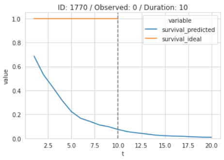
In case the event didn’t occur, the ideal curve would be 100% until the point of censoring. Beyond that point is uncertain:
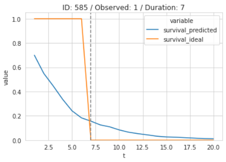
In case the event did occur, the ideal curve would be 100% until the event occurs and zero afterward:
One common metric used for this problem is the Time-dependent Brier Score. This is a Survival adaption of the Brier Score or Mean Squared Error (see sklearn implementation).
The Brier Score can be easily calculated for a single observation where the event was observed. In this example, the score typically moves in the opposite direction of the predicted curve until the event is observed. In this case, the predicted probability was already quite low at the event occurrence, and therefore, the loss drops dramatically:
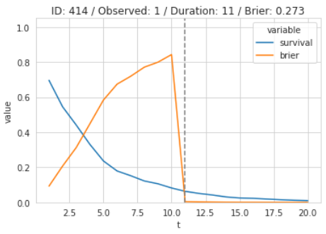
This metric has some disadvantages:
- It can only be calculated for a single observation if the event was observed. For censored cases, it uses a grouped approach, which makes it harder to understand and communicate
- Brier depends on duration, i.e., observations with longer durations usually have a worse score and vice versa
There are other metrics (e.g., Dynamic AUC), but I haven’t found a satisfying and easy-to-communicate metric to evaluate the quality of a predicted Survival curve in the presence of censoring.
The Shape of the Survival Curve
The quality of the curve is measured against the event’s occurrence, but this might not tell the whole story. Different models might produce differently shaped curves (magnitude, rate of decline, drops at certain times) that could be very close in quality metrics. Therefore, it is helpful to visualize and quantify the shape of the predicted curves.
TODO Here are some things to look out for:
- Magnitude: Some models might produce more optimistic curves than others
- Rate of decline
- Curves (within subgroups) dropping to 0 after some point in time: This means that no event prediction can go beyond this point and might be a sign of insufficient training data for this feature combination
- Sharp drops due to cycling appearance of events, e.g., yearly customer subscriptions or election cycles (in a four-year election cycle, there should be a significant decline in the Survival Rate after t=5, t=9, etc.)
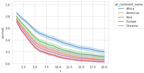
A very basic thing is plotting the average of curves overall and for subgroups of interest. This example shows that the model predicts African governments to rule longer than European ones. The confidence intervals show that the spread in African governments is less stable than in Europe:
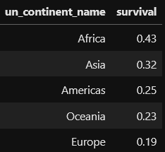
To quantify the magnitude of the curves, we can calculate the Area under the Curve (AUC). This approach can summarize the plot above:
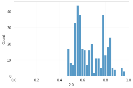
Visualizing the prediction distribution at a specific time can show whether curves are higher or lower than expected. For example, when we have a look at the predicted probabilities for the first year, we can see them already dropping below 60% for a lot of observations, and we might ask ourselves if this is realistic after only one year of government rule:
The shape of the output curve can be important for model selection, but it is hard to put into metrics. Here is an example of how different curves can look per model, which might be a different story than the actual quality metrics:
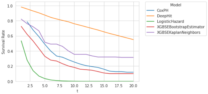
For Logistic Hazards, the average curve drops to zero after about eight years. That would mean that no government goes beyond ten years, which doesn’t seem like a useful prediction.
DeepHit shows a linear decline, while the remaining three models have a sharper decline in the first years which then flattens. This might be more sensible since a government has a higher risk initially, which flattens after a successful start.
Dynamic Model
So far, we have looked at models predicting Survival Curves from the starting point of an observation (e.g., the start of government reign). Let’s call this a Static Model.
In real-world projects, we can update Survival Curves over time by processing new information (e.g., passed reign duration, approval ratings, current polls, scandals, etc.). Let’s call this a Dynamic Model.
The code for this section can be found here.
Static vs Dynamic
The following table summarizes the differences between these two approaches:
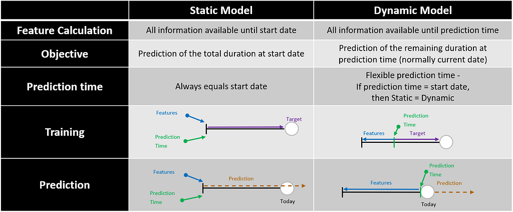
The Static and Dynamic approaches can be applied to all time-dependent models (e.g., time series). As we can see in the overview above, we need to create some split during training in the dynamic scenario to simulate the prediction time. In Time Series, we could split every observation at the desired prediction horizon (e.g., three months). This does not work for Survival since a fixed prediction split already leaks information about the duration target. Therefore, we need to devise another way to split the data.
Splitting
What are splits
In general, there are two types of splits for our data:
- Evaluation split: Split the data into training and evaluation sets — this is what we always do
- Dynamic split: Split the observations along their time dimension and calculate the features at the split point (e.g., use the first five years of a government reign as feature input to predict beyond that point)
Consider this example with the reign of six different governments:

How can we apply the Evaluation and Dynamic Split here? Let’s first look at the Static Model.
Static
In the static context, the time-dependent split is not applicable since we always predict from the start point. The splitting into training and testing is as expected.
For the Random Evaluation Split, we put a randomly drawn subset (e.g., 20%) into the test set:
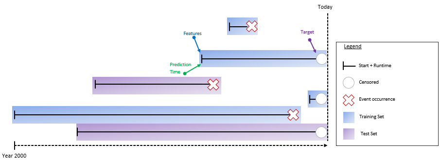
This has the advantage that it mixes in older observations, which we still might want to predict and therefore evaluate.
A second possibility is a Time Evaluation Split where we put every observation that starts after a certain split point into the test set:
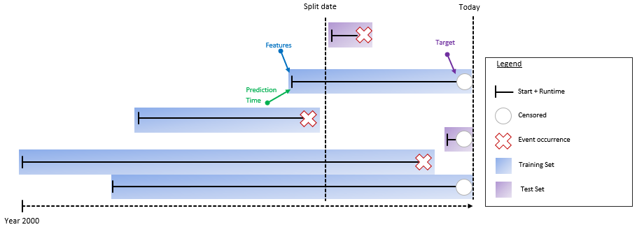
This focuses on the evaluation of newer observations. Depending on the chosen split point, there might need to be more data to evaluate and the split point needs to be pushed back further.
Since these splits are well known, I will not include them in the following dynamic explanation and will focus only on the time-dependent split.
Dynamic
For the dynamic case, the split point can be anywhere between the start and end of the observation. For prediction, we are usually interested in the event probabilities starting from today, but during training, we need to create an artificial prediction point.
There are different ways to do this. The first approach I saw implemented was a fixed time split which splits all data at the same point to simulate “today”:

The fixed time split has certain disadvantages:
- Data loss: Only data that starts before the fixed point and goes beyond can be used. Everything else needs to be thrown away! In the chart above, these observations are marked as Removed
- Fixed prediction horizon of the model defined by prediction point to today
Here is a table with example data where the split is calculated in the year 1988. The column split_time (split_year-start_year) will become a new feature and duration_split (duration-split_time or end_year-split_year) will be the new duration target:
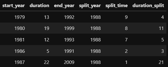
Let’s come back to the data loss: If we are interested in a 20-year prediction horizon, we have to split at the year 1988 (data ends in 2008, normally this would be today – prediction horizon). We have to throw away all data where 1988 is not between the start and end year, leaving us with only 8% of the data!
To overcome these disadvantages, I came up with a Random Split where each observation gets split at a random point between the start and end date:
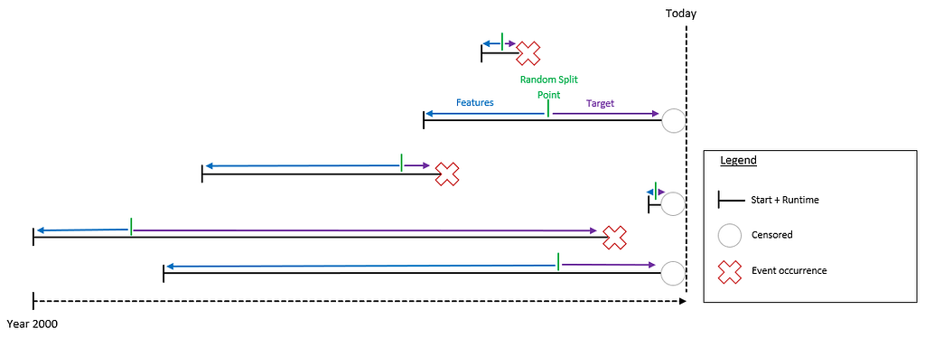
Here is a table with example data where split_time is a random integer between 1 and its duration. As mentioned above, the column split_time will become a new feature and duration_split (duration-split_time) will be the new duration target:
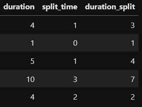
Advantages
- All data can be used regardless of the start time
- Flexible prediction horizon of model
- Allows you to use some form of data augmentation
- Reuse observations at different split points
- Recommended to especially add observations starting at split time 1 to increase Survival Times in Training. This counters the risk of lower predictions due to lower duration targets
We can see from these examples that not only the feature calculation depends on the split, but also the duration target changes while the event target stays the same.
Dynamic Features
In addition to all the Static Features (e.g., the continent or government type), we should add Dynamic Features to improve the model. Here are some examples:
- Reign duration: As we saw above, we get a Dynamic Feature for free when we are splitting along the time dimension (split_time). In this example, this would be the already passed duration of the government’s reign. This feature alone might have a strong impact on the prediction (see example in Dynamic Evaluation below)
- Current polls and approval ratings
- Local elections
- Scandals
Some features can be static and dynamic, e.g., we can include approval ratings at the beginning of the start time and at the prediction point. When using Deep Learning, we can go even further and add whole sequences (e.g., the approval ratings of the last n months) using an RNN architecture.
Keep in mind that the calculation of Dynamic Features requires historization (except for split_time) of all data to get the correct values at the split point.
Dynamic Evaluation
Evaluation complexity increases in the Dynamic Model depending on the prediction horizon. If our horizon is 20 years and we want to update our predictions yearly, then this results in 20 Survival Curves per observation (e.g., government). Now we need to ensure there are valid predictions at every t, not just at the start, as with the Static Model.
We can simulate predictions at different times by replacing the split time feature. The first chart shows all predictions at different times starting at the same point, while the second one plots the actual starting points:
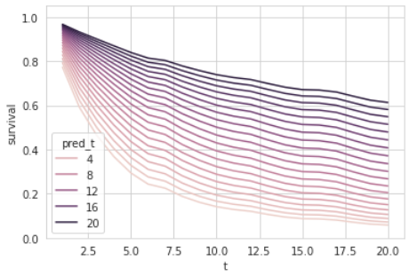
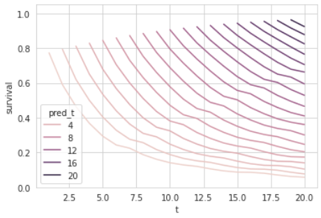
We can observe that the Survival Curves get higher with increasing split times. This makes sense since more and more time is passed with the government still in power, and therefore, the prediction from that point gets more optimistic.
Keep in mind that this intuitive effect will be harder to observe when more dynamic features are involved, which might also negatively affect the curve (e.g., scandals).
Conclusion
I hope this article managed to give an insight into the relevance and challenges of Survival Models. To summarize, here are the three main challenges I see in this field and how this article hopefully contributed to tackling them:
- Education: Inclusion in Basic Data Science courses and popular libraries (scikit-learn, fast.ai) to spread awareness and make it more accessible. In addition, more deep-dive content is needed that goes beyond the fundamentals. This is the type of content I tried to create with this article
- Evaluation: Focuses too much on a single ranking metric (Concordance), which in my eyes is not sufficient. There is a general lack of intuitive metrics to evaluate the quality and shape of the Survival Curve. My article gives some examples of visual inspection and advice on what to look out for to mitigate these issues
- Dynamic Models: Updating predictions over time gets very complex and even harder to evaluate (better evaluation methods could mitigate this). Unfortunately, there are almost no resources to learn about this topic. I talked about the special challenges of Dynamic vs Static Models for Survival, discussed different splitting methods, and gave examples for visual evaluation to mitigate complexity. Most of this content I haven’t found anywhere else.
Data science is a big field with numerous areas, and it shouldn’t be our ambition to understand everything in detail. But having broad basic knowledge is key to translating business problems into suitable data problems and therefore delivering successful projects. I hope I can contribute to this article to gain more appreciation for Survival Models, and there will be more content in the data community in the future.
Survival Models: An Underappreciated Tool for Data Scientists was originally published in Better Programming on Medium, where people are continuing the conversation by highlighting and responding to this story.