Training an AI Model on the Latest Intel Xeon CPU with PyTorch 2.0

Obtaining an accurate “picture” of the subsurface is not as simple as snapping a picture on a smartphone. Seismic exploration is a key component in creating images of the subsurface and finding essential minerals, oil, and gas. Building images of the subsurface is akin to ultrasound technology used to image the human body.
One of the key distinctions in the seismic experiment, however, is that we usually only have access to the very top of the surface, whereas, with an ultrasound, we can survey around the full body. One of the best-known physics-based methods to create geologically-accurate images of the subsurface is called full-waveform inversion (FWI). It is a process by which we can take raw seismic data and, through applying an iterative physics-based approach, recreate the velocities of sound waves in the subsurface (which can be understood as an image).
However, one of the challenges of this physics-based approach is that it is computationally expensive, and it typically relies heavily on a good initial velocity model that is close to the answer. In this article, I will walk you through how I quickly trained a neural network with PyTorch 2.0 on the latest 4th Gen. Xeon CPU, going directly from seismic data to a subsurface model and bypassing the need for an accurate starting model.
Introduction to the Data
The data and methods are taken from the paper OpenFWI: Large-Scale Multi-Structural Benchmark Datasets for Seismic Full Waveform Inversion (Deng et al., 2021). The authors also have released an OpenFWI website here with tutorials, data, and code.
The dataset I used was the entire FlatVel-A, taken from OpenFWI, which is open-source and can be downloaded from their Google Drive. FlatVel-A is taken from the “Vel Family” of datasets that Deng et al. (2021) generated synthetically. The dataset can be used in a supervised deep learning process and comes in pairs: a) the velocity model (image) — the target variable, and b) the seismic shot gathers the feature data.
The FlatVel-A dataset is meant to depict flat-lying sedimentary layers in the subsurface. Figure 1 depicts the data’s process: first, generating the velocity model mathematically, followed by forward modelling the seismic data with a discretized wave equation from the velocity model.

The parameters of the seismic forward modelling can be found in Table 1, and more detailed descriptions can be found in the appendix of Deng et al. (2021). Absorbing boundary conditions are used to suppress unphysical model-edge reflections.

In the dataset, there are 60 model numpy array files (model[1–60].npy) and 60 associated seismic numpy array files (data[1–60].npy). Each model numpy array contains 500 individual velocity models, so in this dataset, there are 500 * 60 = 30,000 models. Each model has five associated seismic shot gathers associated with it, for a total of 150,000 shot gathers. Figure 2 shows the first sample model from model1.npy. The model is square (700 m by 700 m) and has 70 grid points in each direction.

Figure 3 shows a wave propagation animation with the five actual placed source locations on the model’s surface.

Figure 4 shows the forward modelled seismic shot gathers from the velocity model shown in Figure 2. The source positions along the surface are at 0 m, 175 m, 350 m, 525 m, and 700 m. The waves were propagated for one second.

Figure 5 shows the first sample of the velocity model in each of the 60 model files. These velocity models are sometimes called “layer-cake” models due to their simple layer-over-layer structure. In true geological environments, the subsurface can, of course, be much more complex, but in many flat-lying sedimentary environments, it is not entirely unrealistic to have a simple layer-cake geologic structure. However, the very near-surface (first 100 m) is often more complex.

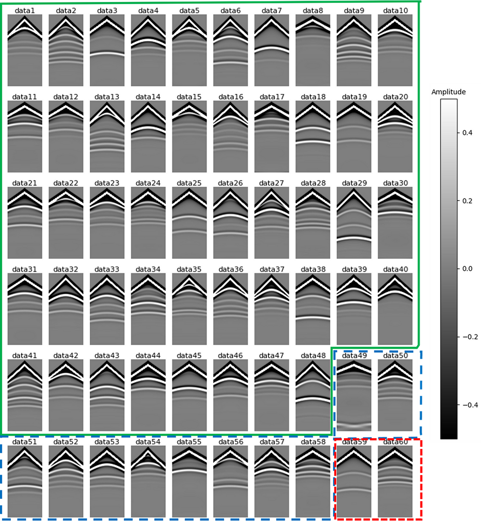
Figure 6 shows a corresponding forward-modelled seismic shot gathers to each model in Figure 5 from the top middle source position.

Training the Model — InversionNET
The algorithm used during training was InversionNET, which is an encoder-decoder CNN neural network (Figure 7). The implementation details can be found in Deng et al. (2021).

In the original paper, Deng et al. (2021) used a single NVIDIA Tesla P100 GPU for the fine-tuning training and trained for 120 epochs on the InversionNET model. In this study, I trained for 50 epochs, used a single bare metal 4th Gen. Intel Xeon CPU, and parallelized over 32 cores. To achieve this, the only change I needed to make was by
1) installing the CPU version of PyTorch 2.0:
pip3 install torch torchvision torchaudio --index-url https://download.pytorch.org/whl/cpu
and
2) running the training script with the torch.backends.xeon.run_cpu command, and specifying the number of cores:
python -m torch.backends.xeon.run_cpu --ninstances 1 --ncores_per_instance 32
--log_path ~/10_data_and_models/FlatVel_A/model_checkpoints/flatvel-a/11/logs/cpu_logs/
    ~/OpenFWI/train.py -d cpu -ds flatvel-a
    -ap split_files -t flatvel_a_train_ben.txt -v flatvel_a_val_ben.txt
    -o model_checkpoints -l model_checkpoints -n flatvel-a -s 11
    -m InversionNet
    -b 256 --lr 0.0001 -eb 10 -nb 12 --workers 1
    -g1v 1 -g2v 0
    --tensorboard
There are four built-in improvements that Intel has contributed to the release of PyTorch 2.0:
- TorchInductor
- GNN
- INT8 Inference Optimization
- oneDNN Graph API
These are outlined in good detail in an article by Susan Kahler on the Intel website: Celebrate PyTorch* 2.0 with New Performance Features for AI Developers.
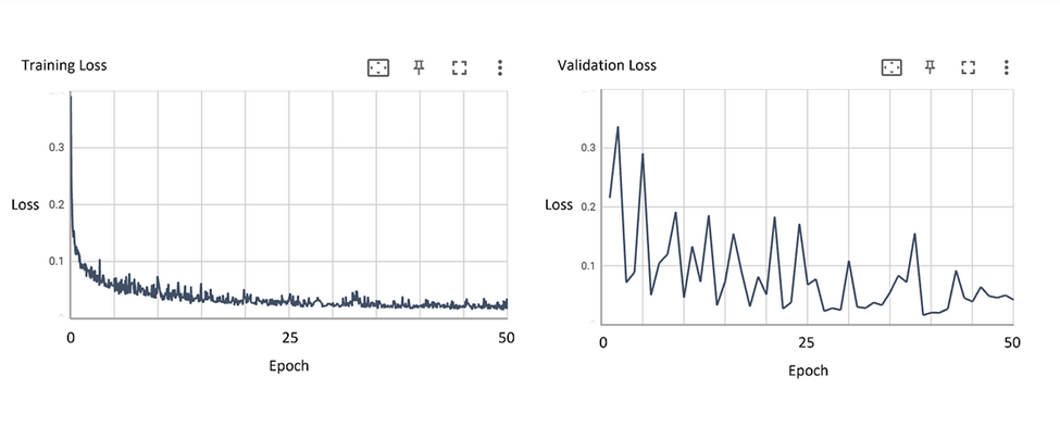
I trained on model[1–48].npy and data[1–48].npy, and used validation data of model[49–58].npy and data[49–58.npy]. Figure 8 shows the training loss and validation loss curves decreasing over time across 50 epochs, a good sign that the model is converging. I used the same training parameters as the original paper, except for only 50 epochs instead of 120: “We employ AdamW optimizer with a weight decay of 1 × 10⁻⁴ and momentum parameters β1 = 0.9, β2 = 0.999 to update all models. InversionNet’s learning rate is 1 × 10⁻⁴, and no decay is applied. The size of a mini-batch is 256.” (Deng et al., 2021)

Sample Predictions From the Trained Model
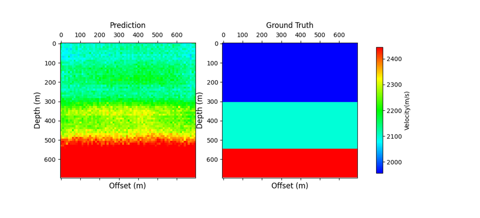
I withheld model[59–60].npy and data[59–60].npy for an unseen test dataset. Figure 9 shows the prediction vs. the ground truth for one of the models after one epoch. The input is a seismic shot gather, and the output is a velocity model image. The prediction does not do very well compared to the ground truth model here but does begin to reflect the layered nature of the model.

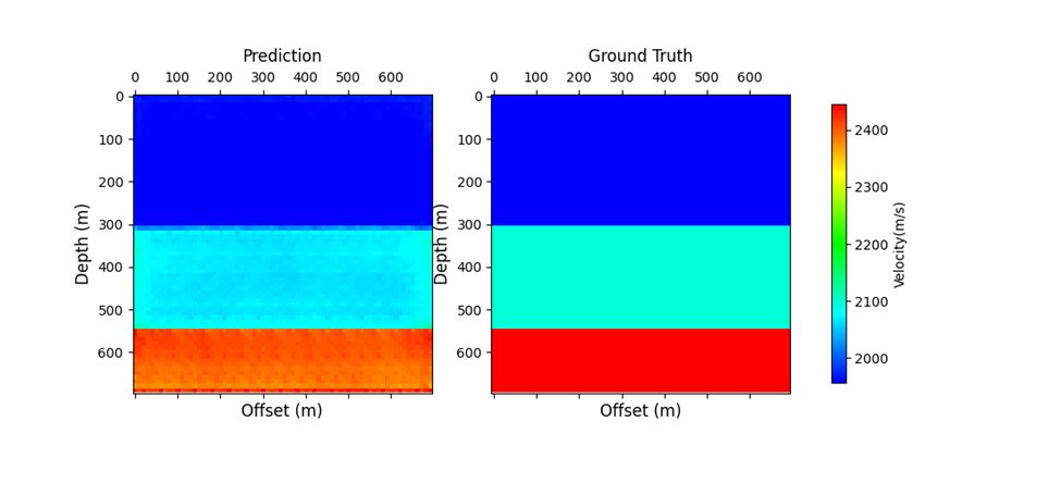
Figure 10 shows a prediction vs. the same ground truth model after epoch 50. We can see that after model training, the model predicts much more closely to the structure of the true model.

Deng et al. (2021) outline three metrics that they considered to evaluate the success of their approach: mean absolute error (MAE), rooted mean squared error (RMSE), and structural similarity (SSIM). For a detailed look at the metrics, please refer to their paper.
Discussion and Limitations
The idea of substituting the physics-based, wave-equation FWI workflow with a purely data-driven deep learning approach is feasible from this study. We could see quite an accurate prediction of an unseen velocity model (Figure 10) from synthetically generated seismic shot gathers, without telling the model anything about the physics of the subsurface. However, the current study has one clear limitation: generalization to other data. It is clear from this study that the AI model does well on structurally similar models (flat “layer-cake” images) and the associated synthetically generated seismic shot gathers.
However, the model’s generalization ability would be severely limited in more challenging and realistic geological environments. To overcome this challenge, field data from a wide array of surveys and supplemental synthetically generated data from a wide variety of geological scenarios would need to be incorporated into the input dataset to obtain a model that generalizes well.
Conclusions and Future Directions
I trained the InversionNET encoder-decoder CNN model on the full FlatVel-A dataset from OpenFWI on a 4th Gen. Intel Xeon CPU to go directly from seismic shot gathers to a subsurface velocity image, without the need for an accurate starting model. Though most deep learning fine-tuning tasks are completed on GPUs, I could complete this fine-tuning task on a CPU. In the traditional physics-based approach, a close starting model is necessary to get to the “answer” and presents a difficult challenge to imaging the subsurface.
In the data-driven approach and without defining the physics, the model converged in 50 epochs to a solution that led to accurate predictions of velocity images for these layer-cake examples.
In the future, I aim to spend more time on incorporating more data that would help the model’s ability to generalize to datasets with a wide variety of structures and to improve upon the performance on CPUs with other optimizations.
Thank you to the tremendous work by Deng et al. (2021) and the Los Alamos National Laboratory (LANL) group for making this dataset and these methods available to the public. The complete training code can be found on the OpenFWI GitHub repository at this link.
Thanks for reading.
I encourage you to check out Intel’s other AI Tools and Framework optimizations and learn about the open, standards-based oneAPI multiarchitecture, multivendor programming model that forms the foundation of Intel’s AI software portfolio.
For more details about 4th Gen Intel Xeon Scalable processor, visit AI Platform where you can learn about how Intel is empowering developers to run high-performance, efficient end-to-end AI pipelines. Information about the Intel Extension for PyTorch can be found here.
Want to Connect?

Get in touch with me on LinkedIn if you have any questions.
Seismic Data to Subsurface Models with OpenFWI was originally published in Better Programming on Medium, where people are continuing the conversation by highlighting and responding to this story.