NBA Games Outcome Project — Web Scraping With Python
How to get data from the NBA seasons’ games and store them for practical use

Motivation
Hello! As I became a big fan of the NBA scene recently and knew my friends and I would be happy knowing the results of previous games, I immediately started thinking of an NBA data science project.
Also, I thought it would be nice to challenge myself to learn something new, and that’s when web scraping came to mind. It has the bonus of giving this project a ‘start completely from zero aspect,’ which is excellent since the project would be more robust, thus, helping me in my journey to becoming a data scientist.
This is the first chapter of a series where I build an end-to-end application whose main purpose is to predict the game outcome between two chosen teams in the pool of 30 NBA professional teams. I am doing this series mainly to show the key aspects of what helped me in doing this project, as I learned a lot in the process, and I believe that knowledge should always be shared.
The Place To Explore and the Relevant Tools I Used

The first step toward this goal was to decide which tools we needed to get the data and where we would explore.
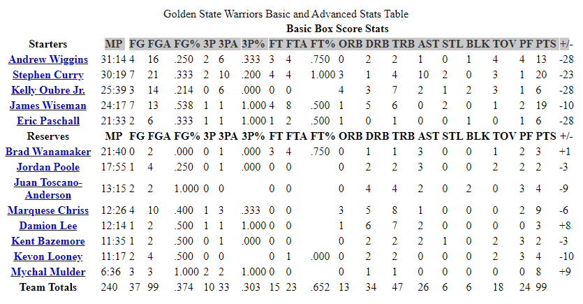
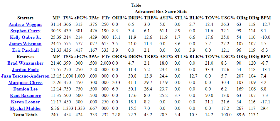
I explored https://www.basketball-reference.com, a great public access domain with NBA seasons’ data ranging from the year 1946! The data I needed was within the boxscores. It contained the basic and advanced stats of a single game.
Python is a great language and has lots of libraries. Even for scraping, we have many options. For this project, I used playwright to go through the seasons’ HTML data.
Playwright supports all modern rendering engines, including Chromium, WebKit, and Firefox. Besides, it can be run on Windows, Linux, and macOS. With this library, I could open the web page and select the exact tab I needed for that domain.
I also used the library BeautifulSoup and some basic frontend knowledge to pull data from the HTML I obtained from playwright. To deal with the HTML files we stored locally, I used the Zipfile library to compress data. It lets you quickly compress and extract your data.
To parse the stored data, I used Regex, a great library to get exactly what you need to work on a text, and mostly, the almighty Pandas, one of the most famous Python libraries for data analysis/manipulation. Finally, I used SQLite to store the data because it efficiently deals with lots of data.
Objective
This process aims to store a dataframe where the columns would contain the basic and advanced stats for each team (the last row of tables shown in the images below). It also showed the opponents’ stats that played against the former, located in their respective boxscores. Additionally, I added these columns for the best individual stats for each team as new columns, but this was entirely optional. So each row would display the full stats of each team per game. Last but not least, I added a column representing whether the team won or not.
Pheww, that’s a lot of variables!


The Methods

First, I got the HTML data files for each season’s month. With playwright, this came with hyperlinks of all boxscores using, and I pulled the data out with BeautifulSoup and stored it locally.
If you are on Mac or Linux, you could code everything in Jupyter Notebooks using the async_api class from playwright. You can do this because the events would run asynchronously, and async allows the code after it to execute immediately. But for Windows, we need to use the sync_api class on a .py file and run it synchronously. Otherwise, it causes errors.
For this, I manually specified the seasons I wanted to scrap. Then, I used the same method again to store all the HTML files of each boxscore, but this time, using the URLs in the files I previously stored.
I could go with the scraping process just once, but I did it this way because it guarantees we will get the right URLs for each box. This makes the process less error-prone and saves the list of paths we already downloaded, so we do not need to get all the data again if the process fails or we want more data from other seasons.
With the boxscores files in hand, the final step was to parse the data with Pandas. This step would ensure the data was ready for the project’s next step. I wanted each feature row to have complete stats per team, so each row needed basic and advanced stats, per team totals, and best individual stats. It also had all those stats from the team’s opponent.
In this process, I also used Regex to get the seasons associated with each boxscore on the HTML file. This step also tracked the data we had already parsed, so we didn’t need to parse everything again if we ran the notebook for new data.
Finally, as the file is complete with all the game stats of the seasons I chose, I stored it in an SQLite database. Besides getting our data in and out quickly, we can append new data if we scrap seasons. For instance, if we wanted to erase data, we wouldn’t have to store it all again.
Results


As the images show, we end up with 152 columns, our features. Each scraped boxscore adds two rows containing data from one game but played by two teams. As the recent regular seasons go from October to April, and about fifteen games are played every two days overall, you can imagine these tables have the potential for dozens of thousands of rows, which is awesome!

Final Thoughts
This project was a lot of fun! I knew it would be challenging initially, but I couldn’t have imagined that I’d learn so much during the process — and handle all the little details that came with it. It was a very rewarding feeling to now have the power to scrap data directly with programming. Even more so on the rich data of NBA stats! The next step would be to explore and analyze this data to get some predictions going.
All the code is explained, and the associated libraries are in my GitHub project folder. Any suggestions are welcome.
Thanks for reading!
Want to Connect?

Feel free to reach me anytime through my LinkedIn.
NBA Games Outcome Project — Web Scraping With Python was originally published in Better Programming on Medium, where people are continuing the conversation by highlighting and responding to this story.