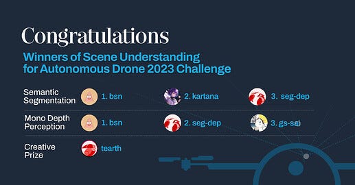
I recently participated in the AICrowd Mono Depth Perception competition, a proud milestone in my machine learning journey. I secured 4th place and was awarded the “Most Creative Solution Award.” In this post, I’ll detail the challenge, my approach, and the lessons learned. I’ve also open-sourced the code and model weights, which can be accessed here — SAUDD2023.

The Challenge
The competition revolved around two key tasks — semantic segmentation and monocular depth perception. These tasks, while similar in terms of model architecture, were different enough to require specific attention. Given the time constraint and my unfamiliarity with the current state of computer vision, I decided to focus on depth estimation.
Depth estimation, simply put, involves gauging the distance between the camera and the objects in a scene. It is a critical perception task for an autonomous aerial drone. Using two stereo cameras makes this task feasible with stereo vision methods. However, the challenge was to develop a model capable of predicting the depth of every pixel using the information from a single camera and a single image.
Dataset
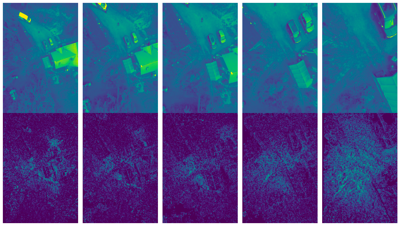
The dataset comprised a series of flight frames captured at specific timestamps by one of the downward-facing cameras on our drones. These images were collected during special data collection operations, not during customer delivery operations.

The dataset included 412 flights, totaling 2056 frames (close to five frames per flight at different Above Ground Levels), complete semantic segmentation annotations of all frames, and depth estimations. The organizers divided the dataset into training, validation, and test (public/private) sets. Although the logic behind this division wasn’t specified, it was likely that the flight id was used for the split.
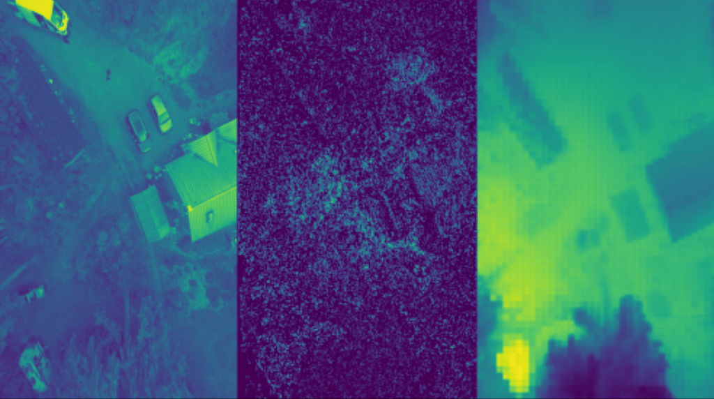
These datasets comprise bird’s-eye-view grayscale images taken between 5 m and 25 m Above Ground Level (AGL). Annotations for the semantic segmentation task are fully labeled images across 19 distinct classes. Annotations for the monocular depth estimation task have been computed with geometric stereo-depth algorithms.
Depth annotations contain relative depth maps, which means the absolute depth value (i.e., in meters) cannot be determined from these maps alone. They are encoded as uint16 images but must be converted into float values representing the depth. Invalid values were represented as zero.

Evaluation Metric
The competition metric is the Scale-Invariant Error proposed in the paper “Depth Map Prediction from a Single Image using a Multi-Scale Deep Network” (section 3.2). The authors observed that simply identifying the average scale of the scene accounts for a significant portion of the total RMSE error. They introduced the SI error that takes into account the global scale of a scene. This metric is sensitive to the relationships between points in the scene, irrespective of the absolute global scale.
For the competition, the metric was calculated individually for each picture and then aggregated using the mean. I implemented this logic as the objective when training the model.

I implemented the same logic as the objective when training the model:
def si_log(prediction, target):
    bs = prediction.shape[0]

    prediction = torch.reshape(prediction, (bs, -1))
    target = torch.reshape(target, (bs, -1))

    mask = target > 0  # 0=missing target
    num_vals = mask.sum(dim=1)

    log_diff = torch.zeros_like(prediction)
    log_diff[mask] = torch.log(prediction[mask]) - torch.log(target[mask])

    si_log_unscaled = torch.sum(log_diff**2, dim=1) / num_vals - (torch.sum(log_diff, dim=1)**2) / (num_vals**2)
    si_log_score = torch.sqrt(si_log_unscaled) * 100

    si_log_score = torch.mean(si_log_score)
    return si_log_score
Validation Strategy
Effective validation is essential in machine learning competitions to estimate a model’s performance reliably without making an official submission. Just like in real-world machine learning applications, the design of the train-validation split ideally should mimic the train-test split (set by the competition organizers or by the nature of the process in the case of real world).
In this competition, each flight was represented by five images, each at different timestamps. My initial strategy was to prevent any leakage by ensuring that different timestamps from the same flight didn’t appear both in the training and validation sets. For this, I employed a KFold split based on flight ids, splitting all flight ids into five folds. This ensured that images from a specific flight id were present either in the training set or the validation set, but not both.
However, this approach did not yield satisfactory results and led to an overestimation of the scores. The exact reasons behind this discrepancy were not entirely clear, leading me to re-evaluate my validation strategy.
I decided to adopt the train/validation split provided by the competition organizers for fine-tuning the hyperparameters of my model and assessing its performance. The KFold split strategy was retained but repurposed to train five different models, with the aim of blending their outputs later. This two-pronged approach allowed me to balance the need for reliable performance estimation and the robustness of the final model.
Image Preprocessing
The preprocessing stage involved loading the images into memory and resizing them to dimensions of 62 * patch_size by 37 * patch_size, where the patch size for DinoV2 is 14. The numbers 62 and 37 were chosen to maintain the original aspect ratio of the images (2200/1550 is close to 62/37). Resizing was carried out using the cv2.resize function (with cv2.INTER_CUBIC used for images and cv2.INTER_NEAREST used for mask depths).
Following resizing, the images were normalized using pre-calculated mean and standard deviation values. These values were computed for each image in the dataset and then averaged.
Given that the input images were single-channel and DinoV2 works with three channels, I replicated the same image three times to mimic the three channels. For the training data, I incorporated some basic augmentations, while validation images were used as is.
self.aug_transform = A.Compose(
    [
        A.OneOf(
            [
                A.HorizontalFlip(),
                A.VerticalFlip(),
            ],
            p=1.0,
        ),
    ],
    p=0.5,
)
The processed image was then passed through the model. The output was resized back to the dimensions of the processed image using the torch.nn.functional.interpolate function. The loss was subsequently computed by comparing the resized depth mask with the output of the interpolation process.
During inference, interpolation was carried out from the model’s output to the original size of the image.
Training Using Cropped Images vs. Resized Images
The dimension of the input images in this competition is approximately 2200*1500. Given this high resolution, it’s not feasible to directly feed the complete images into the network, especially with a visual transformer backbone, due to its quadratic memory complexity. For instance, a single forward pass on a full image consumed over 40 GB of memory.
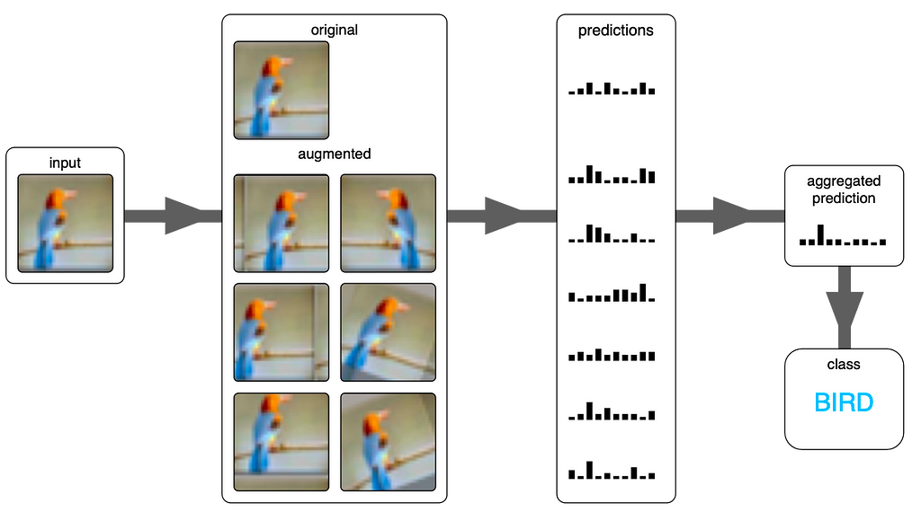
Most depth estimation papers I studied suggest training models using cropped segments of the image, with the alternative approach being resizing the entire image. My initial strategy was to train the model on cropped segments of an image and then perform inference either on the complete image using the CPU or employ test time augmentation (TTA). One of TTA approaches is to use a sliding window to generate predictions on different cropped segments of the image, with the final prediction being an average of all individual predictions.
Training on cropped images seemed to offer two potential advantages:
- Since all images were not the same size, cropping would help maintain the original aspect ratios and avoid distortion from resizing.
- Training with cropped images facilitates easier data augmentation, potentially reducing overfitting.
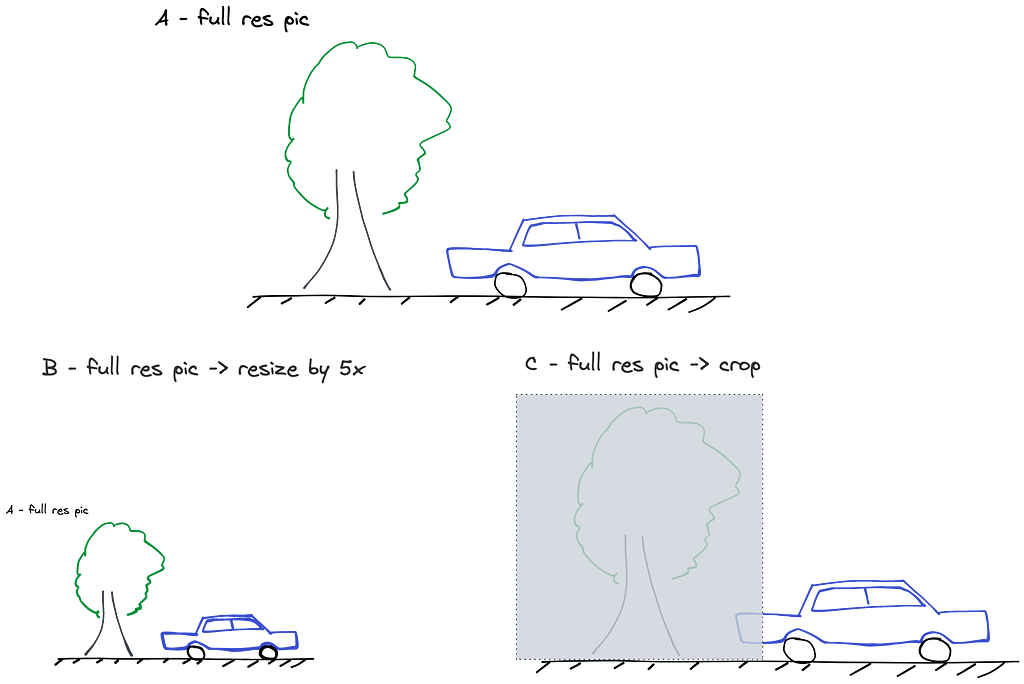
However, contrary to expectations, using cropped images didn’t yield satisfactory results in this competition. My analysis suggests this might be due to the loss of valuable contextual information when cropping. For instance, consider an image with a car and a tree (Image A). When this image is resized (Image B), the model still retains the visibility of the tree, which could be vital for depth estimation of the car. However, if the tree gets cropped out (Image C), this valuable contextual cue is lost, potentially impacting the model’s performance adversely.
Model Architecture
My final solution combined two pretrained models, which were then fine-tuned on my dataset. I utilized the DinoV2 model as the backbone and the head of the MIM model (discarding the SwinBaseV2 backbone of the MIM). The following considerations inspired this approach:
- The MIM architecture performed well for me. During the competition, the DinoV2 paper was released along with its weights. Given the authors’ claims of state-of-the-art performance, I decided to incorporate it into my pipeline.
- While the DinoV2 authors did test their model on a depth estimation task, they only published the weights for the backbone, not for the task itself. They recommended using a depth estimation toolbox (https://github.com/facebookresearch/dinov2/issues/46), but I encountered issues with library version discrepancies during installation. Additionally, the toolbox lacked pretrained weights, and I believed that training the head from scratch wouldn’t be the most efficient approach.
Consequently, I opted to merge the best of both models. I employed the DinoV2 large model, comprising 300M parameters, as the backbone, and the MIM Base head, which included an extra decoder block and eliminated the linear upscale layers.
I also experimented with the DinoV2 G model with 1100M parameters and various versions of MIM (large/base). The embedding sizes were:
DinoV2 output sizes:
- Large (L) — 1024
- Grand (G) — 1536
MIM (SwinBaseV2) head input sizes:
- Base — 1024
- Large — 1536
I tested various combinations (L+Base, L+Large, etc.). If the embedding sizes didn’t match, I included a 1×1 convolution to upscale or downscale the output of Dino. The best results were obtained using the Dino large and MIM base models.
Freeze Backbone, Fine-tune Head
In cases where the dataset is rather small, fine-tuning the backbone may not be beneficial as it can potentially lead to overfitting. Thus, a backbone is frequently frozen during fine-tuning, and only a head is fine-tuned or trained from scratch.
If the backbone is frozen, its output will remain constant. The backbone makes up a significant portion of the total parameters of the model. For instance, the DinoV2 backbones I used have between 300 and 1100 million parameters, whereas a simple convolutional head has between 1 and 10 million parameters.
Consequently, we could cache the output of the backbone for each image in the dataset, and then utilize this output instead of routing the features through the backbone. Here is a simplified pseudocode to illustrate this idea:
backbone_model = ...
head_model = ...

# prepare cache - consumes a lot of RAM or disk space
cache = {}
for i, picture in enumerate(dataset):
    features = backbone_model(picture)
    cache[i] = features

# run model training - much faster
dataloader = DataLoader(dataset)
for batch in dataloader:
    x, y_true = batch
    y_hat = head_model(x)
    loss = clc_loss(y_true, y_hat)
    [...]

# run inference
input_pic = ...
features = backbone_model(input_pic)
answer = head_model(features)
In my experiments, I stored the DinoV2 features on disk, which consumed roughly 100GB of disk space. However, the training process sped up by about five times, making this approach worthwhile.
Unfortunately, the model’s performance was inferior compared to the pipeline where the backbone was not frozen. Hence, I decided not to incorporate this approach into my final solution.
Optimizer: SGD, Adam, AdamW, Adan and Lion
Given the task of fine-tuning, I initially assumed that SGD (Stochastic Gradient Descent) would yield the best performance. During the competition, I experimented with several optimizers, including:
- SGD — Considering the task at hand, it seemed to me that the vanilla SGD would be an ideal choice for fine-tuning.
- Adam — A tried-and-true choice, Adam is a reliable workhorse of optimization.
- AdamW — Given the limited size of the dataset and the mild strength of the augmentations, I thought some additional regularization might be beneficial.
- Lion and Adan — I was also curious to test these modern optimizers.
Based on my experiments, Adan produced the best performance. AdamW and Adan were close runners-up. Lion and SGD, unfortunately, did not yield good results for this particular task.
A concern that emerged was regarding the initial phase of training when Adam’s moments aren’t yet estimated and “steps” could potentially be too large. This might have a negative impact on the model’s performance. To promote stability during training, I incorporated a brief warmup: in the first 200 steps of training, the learning rate linearly increased from 0 to 0.00004.
Accumulated Batch
For training my models, I utilized an A100 GPU with 40Gb memory. Depending on the model and the resolution, the GPU could handle 1 to 6 images in a batch. This led to two notable challenges:
- A small batch size (1–2) resulted in unstable learning.
- Varying batch sizes (e.g., 1 vs 6) led to incomparable results. Smaller batches mean more updates per epoch, making the loss at the end of the epoch an unreliable metric.
To address these issues, I resorted to using gradient accumulation. I set the effective batch size to 12, a somewhat conservative number, but it proved to be effective in my case.
BS = 4
NUM_ACCUMULATION_STEPS = 12 % BS

loss = criterion(prediction, target)
loss = loss / NUM_ACCUMULATION_STEPS
loss.backward()

if n_steps % NUM_ACCUMULATION_STEPS == 0:
    optimizer.step()
    optimizer.zero_grad()
Large Gradients
Throughout the competition, I encountered instances where my model did not converge effectively. I suspected that this issue might be attributed to the problem of large gradients. Large gradients mean large steps that could be made in the wrong direction.
To investigate further, I developed a function to examine the distribution of gradients in each layer. However, due to its slow performance, I executed this check only during every nth epoch of the initial training run, disabling it later for efficiency purposes.
def plot_gradients(model, output_folder):
    gradients = {}
    for name, param in model.named_parameters():
        if param.grad is not None:
            if name not in gradients:
                gradients[name] = []
            gradients[name] = param.grad.cpu().detach().numpy()

    if not os.path.exists(output_folder):
        os.makedirs(output_folder)

    # Plot and save gradient distribution for each layer
    for name, grad in gradients.items():
        plt.hist(np.reshape(grad, [-1]))
        plt.title(f"{name} Gradient Distribution")
        plt.xlabel("Gradient Bins")
        plt.ylabel("Frequency")
        plt.savefig(os.path.join(output_folder, f"{name}.png"))
        plt.clf()
The problem became evident when analyzing the gradients of the last layers of the network. These layers exhibited significantly large gradients, which had a detrimental effect on the convergence of the model. One specific example is the gradients of the output layer, where the magnitudes were notably high.

I addressed this issue by applying a technique called gradient clipping. By implementing gradient clipping, I restricted the magnitude of the gradients to prevent them from exceeding a certain threshold. This approach helped alleviate the problem of large gradients in the last layers of the network and contributed to improved convergence.
clip_grad_max_norm = 3
loss.backward()
torch.nn.utils.clip_grad_norm_(model.parameters(), clip_grad_max_norm)
optimizer.step()
optimizer.zero_grad()
Conclusion
In conclusion, participating in the AICrowd Depth Estimation competition was an enriching experience for me. I achieved 4th place overall and was honored with the “Most Creative Solution” award.
The competition pushed me to explore and experiment with different techniques and strategies. While I encountered challenges along the way, it was a valuable learning experience. I am proud of the results I achieved and grateful for the opportunity to contribute to the field of depth estimation.
My Journey with Depth Estimation was originally published in Better Programming on Medium, where people are continuing the conversation by highlighting and responding to this story.