Enhance your comprehension of conics and gain knowledge on how to fit an ellipse from a collection of 2D points

Introduction
Goal
Any geometric primitive (hyperplane, circle, ellipse, line, …) can be defined by a set of parameters, e.g., radius and 2D center for a circle. Fitting such a model means recovering the more plausible parameters based on the input data points.
When working with a hyperplane, the parametrization is relatively straightforward and can be easily incorporated into an equation like the one below. Once we’ve obtained the optimal coefficients (a,b,c,d), we can effortlessly retrieve the hyperplane normal (a,b,c).

On the other hand, optimizing the parameters for a general ellipse, including minor and major axis lengths, center, and rotation angle, involves employing more intricate methods and approaches.
Key Publications
The first algorithms either dealt with fitting general conics or were computationally expensive.
In 1996, Fitzgibbon suggested minimizing the algebraic distance under the ellipticity constraint (Direct Least Square Fitting of Ellipses). This ensures that the optimal conic parameters correspond to an ellipsis and not a parabola, for instance.
Subsequently, in 1998, Halir and Flusser presented a numerically stable variation of this approach (Numerically Stable Direct Least Squares Fitting of Ellipses).
Without a doubt, the second method is the preferred approach. However, for the sake of readability, I will only describe the first method. The second method shares a similar essence but involves more verbose equations, which could potentially overwhelm the reader.
I encourage readers to consult the original publication for a more detailed exploration of the numerical stability.
Public Implementations
Several implementations based on the numerically stable version of Halir and Flusser are publicly available on GitHub:
General Conic Equation
Conics
Conics, or conic sections, are curves formed by intersecting a plane with a cone’s surface. They include circles, ellipses, parabolas, and hyperbolas, as depicted in the image below from the Wikipedia page dedicated to conic sections. Note that the circle is a special ellipse, where the minor and major axes have the same length.

When planes intersect the cone at its vertex, the resulting intersection can be a point, a line, or a pair of intersecting lines. These special cases are known as degenerate conics.
Equation
A second-degree polynomial equation involving x and y, including linear and quadratic terms, can define any conic.

In practice, conic equations are only sometimes expressed in standard form, as some coefficients may be zero, or it may be more convenient to factorize certain terms together.
Let’s look at some specific equations of conics that arise in practical situations.
Parabolas and Hyperbolas
The best-known parabola is certainly formed by the square function’s graph (blue left curve below). The b and c coefficients of the general conic equations stay equal to zero in the case of a degree-two polynomial in x.
It is often overlooked, as it’s no longer a function of x, but we can transfer the squared exponent of x to y to rotate the parabola (orange middle curve below). The square root function corresponds to the positive branch of this curve.
Unlike parabolas, which form continuous curves, hyperbolas, like the graph of the inverse function, consist of two branches extending infinitely (red right curve below). One notable feature of hyperbolas is the presence of asymptotes, whereas parabolas do not possess this characteristic. Asymptotes are imaginary lines that the hyperbola’s branches approach but never intersect.

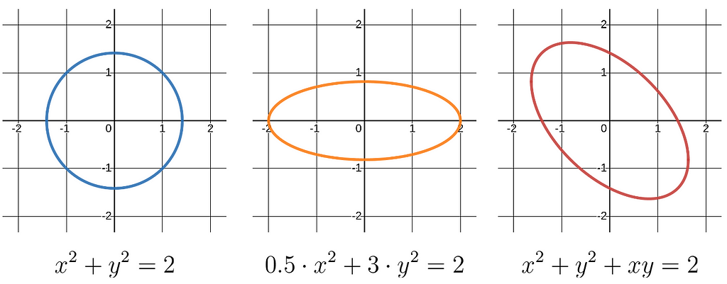
Circles and Ellipses
Both hyperbolas and parabolas are unbounded curves, meaning that they extend infinitely without any endpoint. In contrast, circles and ellipses are closed curves, forming a complete loop without extending indefinitely.
The circle is defined as a set of points equidistant from a central point (blue left curve below). Dilating or shrinking axes, i.e., altering the a and c coefficients in front of x² and y², results in an axis-aligned ellipse (orange middle curve below). The ellipse can be rotated by incorporating a non-zero b value in front of the cross term xy (red right curve below).
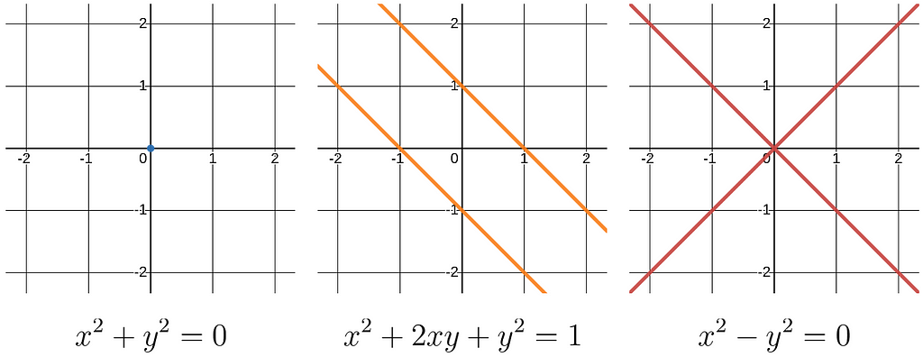
Lines and Degenerate Conics
As said earlier, a degenerate conic might be a single point, a line, or a pair of lines. I’ve not considered the case of a straight line defined like y=x since the general conic equation implicitly assumes that at least one of the quadratic terms is non-zero.
Ellipse Fitting (Fitzgibbon)
Conic discriminant
Similarly to the discriminant of a degree-two polynomial which tells us how many roots there are, we can calculate a conic discriminant which tells us about the nature of the conic. This will help us define a constraint during the optimization to enforce the solution to be an ellipse.
It is easier to approach it through a matrix representation to understand it better. The general conic equation can be rearranged like below using a 2×2 symmetric matrix Q, a 2×1 vector P, and the coefficient f.
This quadratic equation can also be written using homogeneous coordinates.

If the 3×3 matrix A is singular, then the conic is degenerate. When A is non-singular, we can determine the conic type by examining the determinant of the 2×2 matrix Q.

I won’t provide a formal proof, but instead, I’ll offer some intuitive insights before introducing the conic discriminant and its link with the conic type.
In the case of a circle, Q is a scaled version of the identity matrix. In the case of a rotated ellipse, we can transform Q by diagonalization into a diagonal matrix with the squares of the inverses of the minor and major axes (up to a scale factor).
Intuitively, this implies that the eigenvalues of the matrix Q should have the same sign for both the ellipse and the circle. Since the determinant is equal to the product of the eigenvalues, it implies that the determinant of Q must be strictly positive.
Thus, we can introduce the discriminant b²-4ac to distinguish between the conic types. Conceptually, the parabola can be seen as a transition between the ellipse and the hyperbola.

Optimization
The degree-2 polynomial in (x,y) involved in the conic equation is the algebraic distance of a point (x,y) to the conic, which is 0 for a point lying perfectly on the conic. Thus, the optimal conic can be achieved by determining the conic coefficients θ that minimize the algebraic distance.


By constructing a Design matrix, where each row corresponds to the quadratic and linear terms of an input point, we can stack the n conic equations into a unified equation.
While it may be tempting to minimize this equation directly, it is crucial to consider that we seek a specific conic type, namely an ellipse. Therefore, as suggested by Fitzgibbon, it becomes necessary to introduce a constraint that controls the sign of the conic discriminant.
The conic discriminant must be strictly negative to ensure the conic represents an ellipse. To both fix the scale and maintain consistency, we can enforce the discriminant to be -1. Note that this constraint is quadratic in terms of the conic coefficients.

The ellipse fitting problem is constrained minimization with the 6×6 quadratic constraint matrix C.

Introducing the Lagrange multiplier λ and differentiating to find the minimum yields an equation where θ is an eigenvector and λ an eigenvalue.

Remarkably, the positive quantity we‘re minimizing equals the Lagrange multiplier λ.

Since C is rank-deficient, we’re computing the eigenvalues of a singular matrix. Thus, the optimal conic parameters θ are obtained by taking the eigenvector corresponding to the minimum strictly positive eigenvalue.
N.B. Halir and Flusser handle the case where all the points lie exactly on the plane and λ is equal to 0.
Retrieve Ellipse Parameters From the Conic Equation
Introduction
Fantastic! We’ve got our optimal conic coefficients (a,b,c,d,e,f)! But hold on a sec, how in the world do we get the minor and major axes, the rotation angle, and the center from these coefficients?
Ellipse matrix form
Basically, any ellipse can be obtained by taking the unit circle, shrinking or dilating the x and y axes, rotating it, and finally applying an offset. The image below shows how to undo these transforms to map an ellipse to the unit circle, where the conic equation is straightforward, namely x²+y²=1.
N.B. The letter c introduced here stands for the ellipse center and has nothing to do with the conic coefficient c.
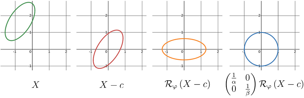
Thus, the ellipse equation can be written as follows, with Rφ being the rotation matrix of angle φ.
N.B. Using a rotation matrix simplifies the equation significantly, avoiding the need to wrestle with numerous sine and cosine terms that would otherwise lead to excessively lengthy and messy equations.
Identification of the parameters
The optimal parameters θ=(a,b,c,d,e,f) is used to build the matrix Q and the vector P of the general conic equation.
By further developing the ellipse equation discussed previously, we can express it in the general matrix form with matrix Q and vector P.

Parameter identification can be performed with an unknown scale factor s.
Ellipse center
Interestingly, the combination of Q and p yields the ellipse center c, effectively eliminating the influence of the scale factor s.

Scale
By leveraging the link between Q and M, we can express the scale s as a function of Q, f, and the newly acquired center c.

Rotation matrix and axis lengths
M, being a symmetric matrix, can be diagonalized in an orthonormal basis. This diagonalization process provides us with both the rotation matrix and the diagonal matrix Σ, which encompasses the inverse square lengths of the minor and major axes.
N.B. The ellipticity constraint guarantees that the diagonal values of Σ are strictly positive.

Fortunately, expressing M is straightforward as it can be obtained by scaling Q with the newly computed scale factor s.
Rotation angle
It is important to recall that a 2×2 rotation matrix can be expressed by using the sine and cosine of the rotation angle φ.
Consequently, the rotation angle φ can be obtained by calculating the arctangent of the elements in the first column.
Since φ covers the entire ]-π, π] range, we have to use arctan2, which is a variant of arctan that chooses the quadrant correctly.

Final Thoughts
We now have all our ellipse parameters.
Conclusion
I hope you enjoyed reading this article and that it gave you more insights on conics and ellipse fitting!
See more of my code on GitHub.
Least Squares Ellipse Fitting was originally published in Better Programming on Medium, where people are continuing the conversation by highlighting and responding to this story.