Unraveling enemy battle plans, one pixel at a time

This weekend marks the eighth and final Battle for Riddler Nation hosted by FiveThirtyEight. The first was held back in 2017. I’m fond of it because I won the second and third, earning me a callout for coming in 18th in the fourth. That was my high water mark, although I did come in 10th in the sixth running. Naturally, I’m looking for any edge I can get for the eighth round, and this is the tale of how my relentless pursuit for such an edge led me to convert RGB values into a wealth of strategic information.

I’ll let Zach Wissner-Gross, who runs the competition, explain the rules:

In a distant, war-torn land, there are 10 castles. There are two warlords: you and your archenemy. Each castle has its own strategic value for a would-be conqueror. Specifically, the castles are worth 1, 2, 3, … , 9 and 10 victory points. You and your enemy each have 100 soldiers to distribute, any way you like, to fight at any of the 10 castles.

Whoever sends more soldiers to a given castle conquers that castle and wins its victory points. If you each send the same number of troops, you split the points. You don’t know what distribution of forces your enemy has chosen until the battles begin. Whoever wins the most points wins the war.

Those familiar with game theory may recognize this as a Colonel Blotto game. You submit a strategy, a list of 10 integers summing to 100, and then your strategy battles with all the strategies other people submitted. Here are some individual results from the previous running to give you an idea (these will come up again).

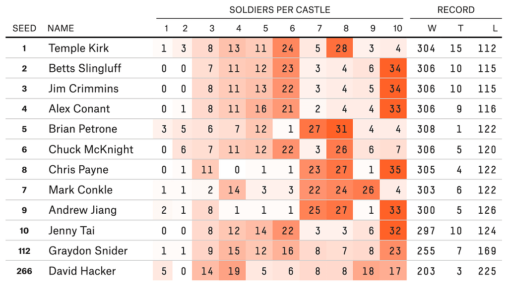
In deciding what strategy to submit, a very helpful piece of information is what strategies have been submitted before. The strategies for the first five rounds are on GitHub, but not those for the sixth or seventh rounds. For our purposes, only Rounds 1–4 and 7 matter; Round 5 had 13 castles, so those strategies won’t translate, and Round 6 allowed “decimated soldiers” — that is, you could assign your soldiers in units of 0.1 — so those strategies won’t help either.

This means we’re only missing one round of data, but it is the freshest data from Round 7. We have the Top 10 strategies from this round above (together with the 112th and 266th ranked strategies because they did well in a knock-out tournament held that round). The only other thing we have is the heatmap Zach posted: “As I have done in previous years, I generated a heat map (with darker orange representing more phalanxes) with all 432 strategies, organized by how well each approach fared in this preliminary stage.”

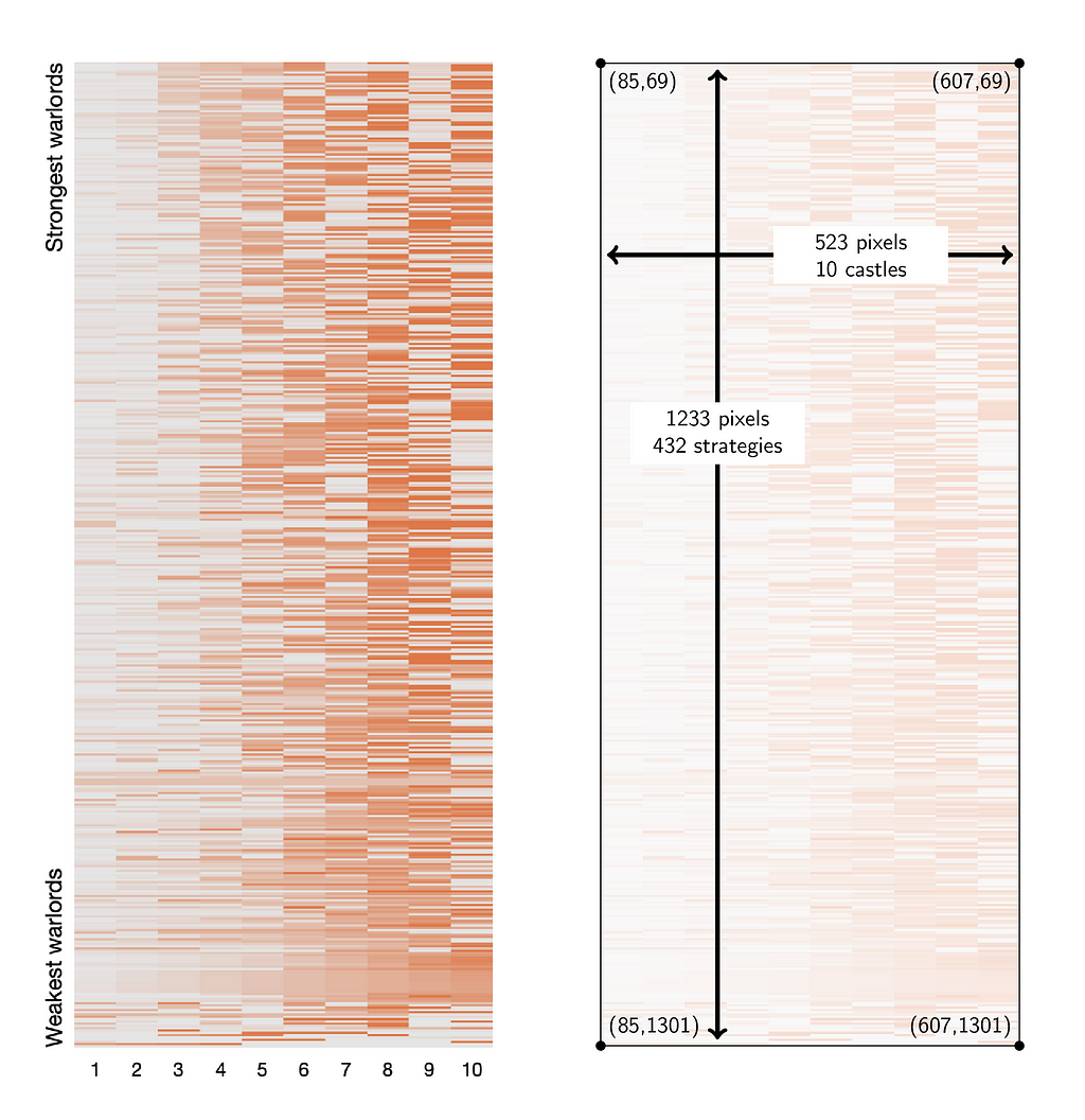
My goal is to reverse engineer this heatmap to recover the strategies.

Question 1: What Pixels Should We Read?

Immediately, we see that this representation is going to be hostile. What I imagine was once a neat and clean data presentation has been contorted to fit into whatever dimensions FiveThirtyEight insists of its graphics. The castles, at least, aren’t too bad. With an average pixel width of 52.3, plenty of room exists to work with. The strategies have been squeezed or squished to an average of 2.85 vertical pixels. These non-integral sizes will be a pain, and it won’t be easy to sample from every strategy precisely once.

Zooming in on the top-right corner of the image can also notice some horrifying (for our purposes, at least) interpolation:

Somehow, we must avoid reading the interpolated rows as their own strategies. Still, the top 10 strategies appear to each get two rows of pixels and be separated from each other by one interpolated row. In the figure below on the right, I have included a rescaled portion of the part of the heatmap that should correspond to the top 10.

Poking around on GIMP, I see that the encoding of the Top 10 is at least fairly nice. Each of these strategies is represented by two vertical rows of pixels, with those two-pixel strips separated from each other by one interpolated row. We can sample the castles starting at x-value 110 and increasing by increments of 53; these segments are wide enough to have lots of wiggle room.

import numpy as np
from PIL import Image

image = Image.open("heatmap.png")
image = image.convert("RGB")
data = np.array(image)

# Top 10 strategies, RGB values
data_top_10 = data[69:97:3, 110:598:53]

# Define the ground truth matrix
ground_truth_mat = np.matrix([
    [ 1,  3,  8, 13, 11, 24,  5, 28,  3,  4],
    [ 0,  0,  7, 11, 12, 23,  3,  4,  6, 34],
    [ 0,  0,  8, 11, 13, 22,  3,  4,  5, 34],
    [ 0,  1,  8, 11, 16, 21,  2,  4,  4, 33],
    [ 3,  5,  6,  7, 12,  1, 27, 31,  4,  4],
    [ 0,  6,  7, 11, 12, 22,  3, 26,  6,  7],
    [ 0,  1, 11,  0,  1,  1, 23, 27,  1, 35],
    [ 1,  1,  2, 14,  3,  3, 22, 24, 26,  4],
    [ 2,  1,  8,  1,  1,  1, 25, 27,  1, 33],
    [ 0,  0,  8, 12, 14, 22,  3,  3,  6, 32]])

We haven’t figured out what to do below the Top 10 yet, and I’ll return to that near the end, but for now, let’s move on.

Question 2: What To Even Measure?

One can make many mistakes in answering this question, and I certainly did. First, I tried measuring the distance between the colors of the pixels and the orange. But what orange? Then I tried to find the “best” orange to use for this, and I found that even the “best” orange still didn’t fit the data very well.

My first good idea was that instead of measuring how close the colors are to orange, I should measure how far they are from gray. There are several 0s in the top 10, so the RGB values of the corresponding pixels will serve as a good anchor. Fortunately, these RGB values are identical (229, 229, 299).

Using this color as our anchor, we’ll replace all our color data with their distance from this color.

gray_rgb = np.array([229, 229, 229])
dist_top_10 = np.apply_along_axis(lambda x: np.linalg.norm(x - gray_rgb), axis=-1, arr=data_top_10)

Question 3: How To Translate to Soldier Counts?

Instead of making the mistake I initially made, let’s be smart and start with a plot, comparing the distance-to-gray of the pixels (of the top 10 strategies) with their ground truth values from Zach’s chart.

import matplotlib.pyplot as plt

# Flatten the distance and ground_truth_mat arrays for plotting
dist_top_10_flat = dist_top_10.flatten()
ground_truth_flat = ground_truth_mat.A1

# Create a scatter plot
plt.scatter(dist_top_10_flat, ground_truth_flat)
plt.xlabel('distance from gray')
plt.ylabel('ground truth')
plt.show()

The best thing we could expect would be a straight line. We almost get that lucky.

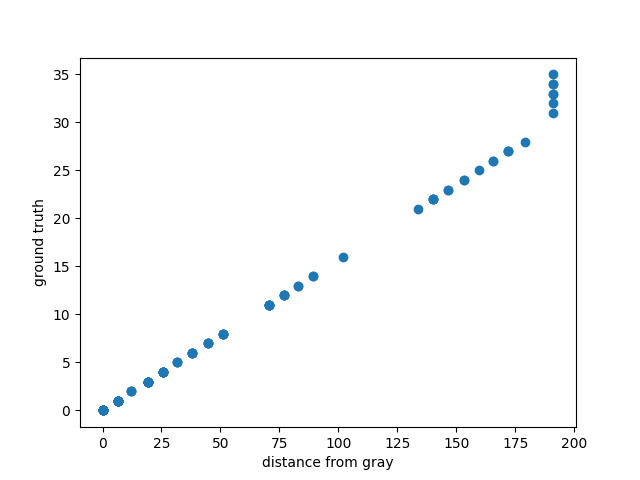
This plot shows that all of the large (31 and up, at least) ground truth values have been squished down, but other than that, distance-to-gray has a nice linear relationship to the actual number of soldiers. This makes sense. If Zach hadn’t squished these values down before he generated the heatmap, it would have been dominated by the dude who put 100 soldiers in castle 1. Fun fact: this is a type of “winsorizing.”

Now we exclude these large ground truth values and find the relationship between distance-from-gray and number-of-soldiers for the values where this relationship is linear.

# Filter the arrays to exclude points where the fit won't work
mask = ground_truth_flat <= 30
dist_top_10_filtered = dist_top_10_flat[mask]
ground_truth_filtered = ground_truth_flat[mask]

# Reshape data for lstsq
A = dist_top_10_filtered.reshape(-1, 1)
b = ground_truth_filtered

# lstsq returns several values, we only care about the first one
slope, residuals, rank, s = np.linalg.lstsq(A, b, rcond=None)

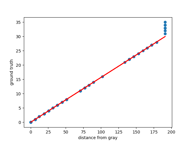
We get a slope of 0.15679897 and residuals of only 0.14377823. We knew the fit was going to be good, and the residuals tell us it is good, but let’s plot it anyway to revel in its accuracy.

line_y = slope * dist_top_10_flat
plt.plot(dist_top_10_flat, line_y, color='red')
plt.scatter(dist_top_10_flat, ground_truth_flat)
plt.xlabel('distance from gray')
plt.ylabel('ground truth')
plt.show()

Question 4: How To Recover the Large Values?

The linear correspondence between distance-to-gray and number-of-soldiers works great until we reach the RGB color (222, 120, 72), at a distance 191.32778707 from gray. This color represents all values 30 and up.

If a strategy has a unique entry of at least 30, we can increase this entry to account for however many soldiers are missing after we round the values to integers. But if the strategy has multiple entries of at least 30, we can do nothing. I will elect to split the missing soldiers equally among those positions, but I am not recovering those strategies faithfully.

def recover_strategy(dist_vec):
    # Given a vector of distances-to-gray, recover the strategy.
    estimated_values = [slope[0] * dist for dist in dist_vec]
    strategy = np.rint(estimated_values).astype(int).tolist()

    # What will cut-off values look like?
    max_rgb = np.array([222, 120, 72])
    max_dist = np.linalg.norm(max_rgb - gray_rgb)
    max_rounded = np.rint(slope[0] * max_dist).astype(int)

    # Get the indices of possibly-cut-off values.
    max_indices = np.where(strategy == max_rounded)[0]

    # Deal with extra soldiers if any.
    extra = 100 - sum(strategy)
    if extra:
        # There are missing soldiers. Do the best we can.
        if len(max_indices) > 1:
            print(f"Missing soldiers and multiple max entries, so have to guess.")
        elif not len(max_indices):
            print(f"Missing soldiers but no max entries, so not fixing.")

        if len(max_indices):
            each_extra = extra // len(max_indices)
            remainder = extra % len(max_indices)

            # Distribute the extra soldiers
            for i in max_indices:
                strategy[i] += each_extra
            for i in range(remainder):
                strategy[max_indices[i]] += 1

    return strategy

To test this, we can apply it to the Top 10.

>>> recovered_top_10 = np.apply_along_axis(recover_strategy, axis=1, arr=dist_top_10)
>>> recovered_top_10 - ground_truth_mat
matrix([[0, 0, 0, 0, 0, 0, 0, 0, 0, 0],
        [0, 0, 0, 0, 0, 0, 0, 0, 0, 0],
        [0, 0, 0, 0, 0, 0, 0, 0, 0, 0],
        [0, 0, 0, 0, 0, 0, 0, 0, 0, 0],
        [0, 0, 0, 0, 0, 0, 0, 0, 0, 0],
        [0, 0, 0, 0, 0, 0, 0, 0, 0, 0],
        [0, 0, 0, 0, 0, 0, 0, 0, 0, 0],
        [0, 0, 0, 0, 0, 0, 0, 0, 0, 0],
        [0, 0, 0, 0, 0, 0, 0, 0, 0, 0],
        [0, 0, 0, 0, 0, 0, 0, 0, 0, 0]])

We’ve perfectly recovered the Top 10. On to the Bottom 422!

Question 5: Which Rows To Include?

The strategies get 2.85 vertical pixels on average, and they are (sometimes) separated by rows of interpolated pixels. We can’t hope to take regularly spaced samples, even though we got lucky in the Top 10.

First, to make everything easier to handle, I’ll convert to distances-to-gray and then check how many unique rows we have.

# Convert to distance-to-gray vectors.
dist_data = np.apply_along_axis(lambda x: np.linalg.norm(x - gray_rgb), axis=-1, arr=data[69:1302:1, 110:598:53])
# Number of unique rows.
unique_rows = set(map(tuple, dist_data))
len(unique_rows)    # Should return 732.

Running this code shows we have 732 unique rows, much more than the 432 strategies we are trying to recover.

At least from the Top 10 data we’ve examined, it seems that at least two rows of pixels represent every strategy. On the other hand, the interpolated rows of pixels should not be like either row they are next to. We start by filtering out the presumed-interpolated rows and checking how many unique rows are left.

# Zero out all rows that are not equal to an adjacent row.
zero_vec = np.zeros_like(dist_data[0])
filtered_dist_data = dist_data.copy()
for i in range(1, dist_data.shape[0] - 1):
    if not np.array_equal(dist_data[i], dist_data[i - 1]) and not np.array_equal(dist_data[i], dist_data[i + 1]):
        filtered_dist_data[i] = zero_vec
unique_rows = set(map(tuple, filtered_dist_data))
len(unique_rows)    # Should return 419.

Now, it says we only have 419 unique rows. One is the zero vector, so we have 418 unique strategies. These should be all the unique strategies in the data set, although some were submitted more than once. The remaining task is to recover these strategies the correct number of times.

We begin by making an initial selection of 432-row indices from filtered_dist_data. We then wiggle these indices to ensure that all final indices correspond to nonzero rows and that we never have two adjacent rows. The code below does this and leaves us with a selected_matrix.

# Select 432 row indices, as equally spaced as possible, from filtered_dist_data.
# Note that filtered_dist_data has length 1233; I played around with where this
# np.linspace starts and stops to get 418 unique nonzero rows.
selected_indices = np.round(np.linspace(0, 1231, 432)).astype(int)

# We will restrict to the nonzero rows.
nonzero_rows = np.unique(np.nonzero(filtered_dist_data)[0])

# Initialize a list to store the final selected indices.
final_indices = []

# To be selected, a row must be nonzero and not adjacent to another selected row.
# If a member of selected_indices fails one of these conditions, replace it with the
# nearest index that does not fail the conditions.
for idx in selected_indices:
    if idx not in nonzero_rows or (len(final_indices) > 0 and abs(final_indices[-1] - idx) <= 1):
        # This index must be replaced.
        nearest_rows = nonzero_rows[np.abs(nonzero_rows - idx).argsort()]
        for nearest_row in nearest_rows:
            if len(final_indices) > 0 and abs(final_indices[-1] - nearest_row) <= 1:
                continue
            else:
                final_indices.append(nearest_row)
                break
    else:
        final_indices.append(idx)

    # Stop if we have selected 432 rows.
    if len(final_indices) >= 432:
        break

selected_matrix = filtered_dist_data[final_indices, :]

Check to make sure that we did not lose any strategies.

unique_rows = set(map(tuple, selected_matrix))
len(unique_rows)    # Should return 418.

The comment in the code making selected_matrix explains that a little fidgeting was involved with getting precisely 418 unique strategies (the number we want). This is a bit about how frequently some of the strategies appear in the data set, but it has all of them, and I believe they are represented with a fairly accurate frequency.

All that remains is to convert these distance vectors to strategies.

recovered_strategies = np.apply_along_axis(recover_strategy, axis=1, arr=selected_matrix)

Since recover_strategy() prints messages when it encounters missing soldiers it can’t uniquely place. I can tell you that of the rows selected by process_data(), there were 47 with missing soldiers and multiple max entries, while 11 had missing soldiers and nowhere to put them.

Moreover, this recovered_strategies matrix matches all of the rows of the Top 10 + #112 + #266 chart that Zach shared.

>>> recovered_strategies[[*range(10), 111, 265]]
array([[ 1,  3,  8, 13, 11, 24,  5, 28,  3,  4],
       [ 0,  0,  7, 11, 12, 23,  3,  4,  6, 34],
       [ 0,  0,  8, 11, 13, 22,  3,  4,  5, 34],
       [ 0,  1,  8, 11, 16, 21,  2,  4,  4, 33],
       [ 3,  5,  6,  7, 12,  1, 27, 31,  4,  4],
       [ 0,  6,  7, 11, 12, 22,  3, 26,  6,  7],
       [ 0,  1, 11,  0,  1,  1, 23, 27,  1, 35],
       [ 1,  1,  2, 14,  3,  3, 22, 24, 26,  4],
       [ 2,  1,  8,  1,  1,  1, 25, 27,  1, 33],
       [ 0,  0,  8, 12, 14, 22,  3,  3,  6, 32],
       [ 1,  1,  9, 15, 12, 16,  8,  7,  8, 23],
       [ 5,  0, 14, 19,  5,  6,  8,  8, 18, 17]])

The End Result

One way to measure the success of this operation is to compute the records of the recovered strategies and compare them to the results Zach posted. Here’s what I get when I do that:

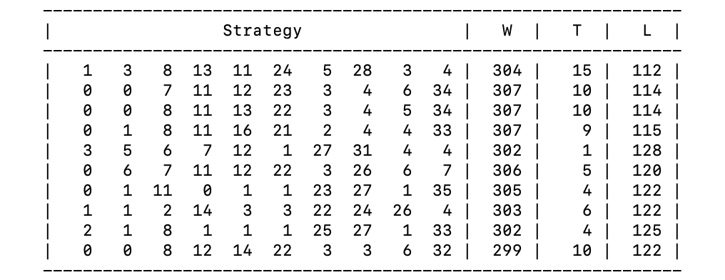
This does not completely align with Zach’s results. The most likely culprit is how I essentially gave up on the 47 strategies with missing soldiers and more than one big entry they could be assigned to. One could imagine using the win-loss-tie records that Zach posted to make more educated choices for where to apply those extra soldiers (by casting the assignment of those 47 sets of missing soldiers as a constraint programming problem, say), but I’ll resist that temptation.

While this shows that I didn’t perfectly recover all of the strategies, I’m reasonably happy with the extracted data set, at least to plan my strategy for the eighth Battle for Riddler Nation. The only thing left is to save the strategies to a CSV file.

import pandas as pd
df = pd.DataFrame(recovered_strategies)
df.columns = ["Castle " + str(i) for i in range(1, 11)]
df.to_csv("castle-solutions-7.csv", index=False)

And then put them on GitHub for anyone to use.

Decoding a Heatmap: Using Espionage in the Battle for Riddler Nation was originally published in Better Programming on Medium, where people are continuing the conversation by highlighting and responding to this story.