So you are training a deep neural network, and it’s slow. But you have multiple GPUs and/or computers available.

How do you utilize them? How do you utilize them efficiently?

This very simple question has a surprisingly complicated answer because it lies at the intersection of multiple fields — General Computer Science (CS), Machine Learning, and Software Systems. But don’t worry, I will give you a beginner-friendly introduction to this problem, focusing on deep learning use-case.

This series of articles is a brief theoretical introduction to how parallel/distributed ML systems are built, what are their main components and design choices, advantages and limitations.

Prerequisites

Basic knowledge of:

• Neural network architectures (e.g. if you know what a ResNet or a Transformer is, that’s good enough);
• Common matrix operations (dot product, convolutions, etc.);
• Backpropagation algorithm;
• General computer science (what’s a GPU, how devices communicate with each other in a computer, what’s an Ethernet port, etc.)

Credits

This article builds on the ML710 “Parallel and Distributed Machine Learning” course that I took at Mohamed bin Zayed University of Artificial Intelligence (MBZUAI) as a part of my Master’s Degree. Some slides from the course were used as illustrations.

Special thanks to Dr. Qirong Ho, the lecturer and Assitant Professor at MBZUAI who developed the course and helped with creating this article.

What makes ML programs special

Parallelizing ML programs is fundamentally different from parallelizing regular CS problems due to their nature.

What do we want to parallelize? Model training — it typically takes most of the time and resources and is the most important part of any ML program. We are going to safely ignore non-training parts, like loading the weights, logging results, etc., since they are not the bottleneck.

What is an ML program? Imagine you’re training a ResNet model on the ImageNet dataset, a typical image classification task. You write your code in PyTorch, run it and you get e.g. 80% accuracy in the end.

That is an example of an ML program — software, which is an optimization-centric program that solves an iterative convergence (IC) problem using local updates. Let’s break this definition down:

Optimization-centric: our program is not just a sequence of deterministic steps (like a graph traversal or a sorting algorithm), but rather a sequence of repeated steps that lead us to an approximate solution (in the case of backpropagation used for the neural network — to a local minimum of the loss function). Think about it like this: a sorting algorithm that guarantees that the numbers will be sorted mostly correctly is unusable. But the aforementioned image classification ML program that outputs a model with 80% classification accuracy is … normal, maybe even good, depending on the problem setting and our accuracy requirements.

Iterative convergence: an ML program is basically a simple loop of the form for t in range(T): A_t = update(data, A_t-1) , where a certain function iteratively updates the model’s parameters (weights) A for T iterations. And when we’ve done all T iterations or when the updates between the iterations become small enough, we say that our program converged. Then we take the trained model and use it.

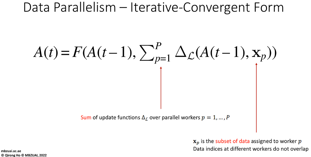
A more formal definition of iterative convergence has the following form:

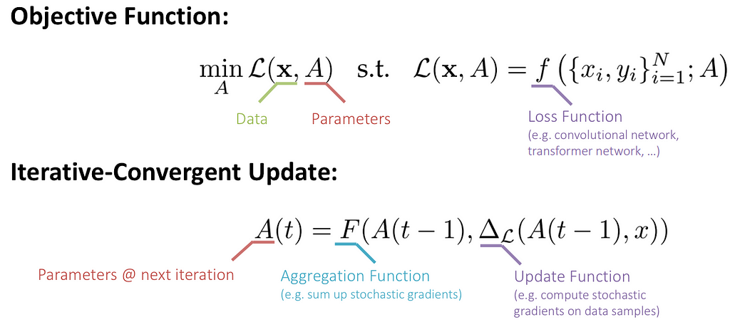
The IC equation is just a recurrent equation, which defines the parameters of the model at training step t given it’s parameters at step t-1 , an update function Δ to compute the step, and an aggregation function F — to aggregate updates from multiple data samples into a single update, that is then applied to the parameters A.

In the case of backpropagation that we use every day, the update function Δ is just negative gradients of the weights (-λ∇A, λ being the learning rate), and the aggregation function F is simply an average of the gradients.

Remember, 1 step = 1 batch, not 1 sample. Since no matter how large our batch is, in backpropagation, we always aggregate the gradients across all data samples into a single vector before making a single step toward the minimum.

Why is this definition important? Because now we have detached from the implementation details of your program — whether you use SGD or Adam, a learning rate scheduler, weight decay, or mixed-precision training — the same parallelization approaches can be applied because it’s still the same equation, regardless of your Δ and F, which capture these details.

A few other interesting properties of ML programs include:

• Error-tolerance — you can have noize and mislabeled samples in your data, ignore some update steps, and still get a well-working model, meaning the algorithm is robust towards limited errors.
• Uneven convergence — the model converges faster in the beginning and slower towards the end (think what happens to |∇A| — the magnitude decreases, i.e. updates to parameters become smaller). Also, not all parameters are equally important and converge at the same speed during training.
• Parameters have structure — particularly, in Deep Neural Networks (DNNs), where we have sequences of blocks/layers with typically rigid structures.

Different techniques we’re going to discuss here later will illustrate and use these particular properties for efficient training parallelization.

Now you see that ML programs are quite different from typical CS programs, so we need new approaches to parallelize them. What do we do?

Three main dimensions of parallelism — classification

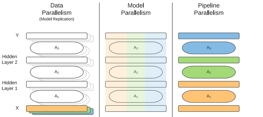
The three main ways to parallelize model training are Data Parallelism, Model Parallelism, and Pipeline Parallelism.

Data Parallelism

Data parallelism is one of the simplest approaches to speeding up model training. It ignores the structure of the model and update function Δ and only focuses on the aggregation function F.

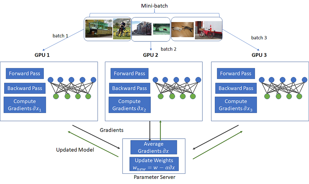
In this approach we split the batch into equal parts and compute the updates for all of them in parallel, one for each worker device/machine that we have. We then gather and add all the updates together, perform a single optimization step, and send the new weights back to the workers to use in the next iteration.

More formally it will look like this: Given p worker devices/machines, and a batch of K data samples, the iterative-convergent formula would look like this:

Each worker only processes K/p data samples, and the optimization step can be performed on either a separate machine/device, or on one of the workers. The model is fully replicated on each worker.

Why it works: Data Parallelism is essentially equivalent to increasing the batch size during training. Larger batch size — more accurate optimization step, thus convergence in fewer steps. And, since the updates are calculated on multiple workers in parallel, fewer steps = less time.

Advantages:

1. Easy to implement, usually has available implementations already — DD and DPP in PyTorch. A good starting point.
2. Fully model-agnostic — works with anything (CNNs, Transformers, GANs, etc.) without modifications.
3. Easy to predict speed improvements before running (e.g. if we use 4 GPUs, then the convergence will be at most 4x quicker).

Disadvantages:

1. Requires the model to fit into the memory of a single worker. But what if it’s really large? Then you have a problem 🙂
2. Scalable only up to a point (without further tricks and optimizations, such as LAMB), as mindlessly increasing batch size reduces the statistical efficiency of each sample inside of that batch (more on that in the next article). Basically the larger the batch size, the more your gradient vector resembles the gradient vector of the entire dataset. If you go from 4 to 8 samples in the batch, you’ll likely get a more accurate gradient direction in your optimization steps and thus will get to the minimum quicker. But if you have e.g. batch size of 1024 samples, then (depending on your problem) it’s likely sufficiently representative of your dataset, and bumping it to 2048 you will just do 2x more computations and arrive in the same place.
3. Relatively large communication payload (if the model has |A| parameters, one iteration requires a total of 2|A|pb bytes to be sent across the devices, where b is the number of bytes per parameter (typically 4 or 2 when using mixed-precision training). For example, if you train a ResNet50 which has ~23M parameters on 8 parallel workers, you will have to send a total of ~1.47 Gb of data per iteration.
   It’s usually fine for GPUs in the same machine, and for multiple physical machines connected through a local network as well, using newer Ethernet standards (10 Gbps+).

Model Parallelism (or “operator-level parallelism”)

It’s all good and well if your model fits in a single GPU’s memory and can do a forward-backward pass on at least one data sample.

But what if it can’t? If there is not enough space on the device to process even a single data sample, we have no choice but to reduce memory usage. What are our options?

1. Reducing the data sample size — e.g. downsampling an image or an audio signal. Not always possible (how do you downsample a sentence?) and typically undesirable due to accuracy penalty.
2. Implementation-specific options — e.g. Quantization or Mixed Precision training. Can be a great tool, but they are not scalable so can only help so much. For example, when using MP you can get up to 2x reduction in memory usage (32bit -> 16bit floating point numbers), but what if you need 4x? 16x?
3. Reduce the model size — of course, choosing a smaller model with fewer parameters is sometimes an option, but often the whole point is to train a big model to get great performance, so the option is not practical.

This is where the Model Parallelism comes in. What we can do instead of all this is reduce the model size per device. How?

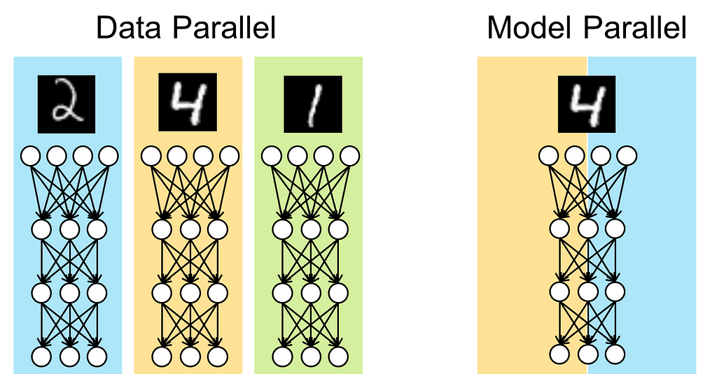
We split some (or every) layer of the model across multiple devices, and each device is responsible for performing forward and backward passes only for some of the model’s parameters.

Examples of layers you can parallelize this way:

1. Linear layer: Given N inputs and M outputs, we have an NxM parameter matrix (biases included). We can slice the matrix vertically, splitting it into k Nx(M/k) matrices, compute their products with BxN input each in parallel, and then obtain k Bx(M/k), concatenate, and get the final output (BxM) (B being the batch size).
2. Convolutional layer — the simplest option is to spread the filters across the devices. Since every convolutional filter is applied independently, having N convolutional filters, we split them into k devices, run k parallel convolutions, and obtain k N/k-channel feature maps, which we then concatenate along the channel dimension, getting a single N-channel feature map.
3. Multi-head attention — since the attention mechanism from Transformer networks consists mainly of a series of linear transformations (i.e. matrix multiplications), these transformations can be parallelized like in pt.1 separately.
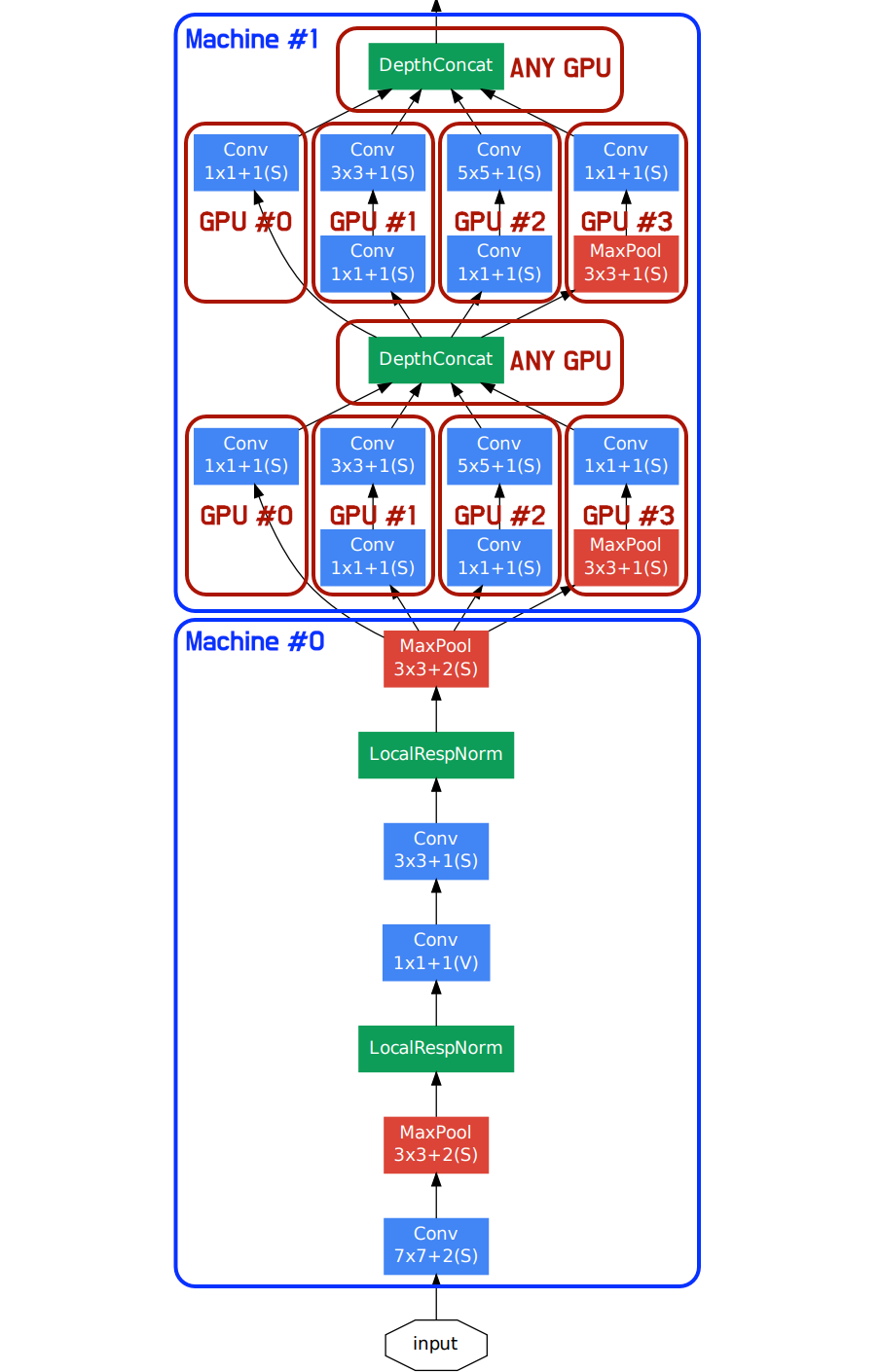
4. Parallel branches — some architectures (e.g. Inception family) have multiple layers executed independently from each other, which you can easily assign to different devices to process (see the Hybrid approaches section for examples)

Operator-level parallelism is a commonly used term when referring to certain types of Model Parallelism when applied to individual mathematical operators (e.g. convolution, dot product, matrix product, interpolation, pooling, etc.) rather than blocks/layers of a neural network or other ML model.

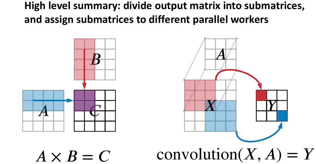
Examples 1–3 are also often called “Operator-level parallelism” or just “operator parallelism”, because they do not always follow the definition of Model Parallelism, often becoming a Hybrid Data and Model Parallelism approach, as illustrated in the figure above.

The figure shows that we can split the matrix multiplication operator across multiple devices in both Data Parallel and Model Parallel fashion. The same goes for a convolutional operator — different devices can process different parts of the input image/feature map with the same kernel and then concatenate the results together. Or you can also have different kernels process the whole image, or even parts of the image, or cut the kernels channel-wise, or even decompose a 3×3 convolution into 2 (1×3 and 3×1) smaller consecutive kernels and apply them in a Pipeline Parallel fashion.

There is nothing special about this parallelism approach, and “operator-level parallelism” is just a convenient umbrella term for it. Now if someone is mentioning “Operator parallelism” you will know what they mean 🙂

Now back to the Model Parallelism — in more scientific terms, every device only processes a subset of the model’s parameters, giving us the following formula:

Sp just refers to a subset of parameters A available to each worker p. For example, if your model has 10 parameters and you have 4 workers, then your parameter index sets Sp could look like this:

1. S1 — {0, 5, 6}
2. S2 — {1, 4, 9}
3. S3 — {2, 3}
4. S4 — {7, 8}

These just denote indices of parameters available to the workers. So workers 1 and 2 would run forward and backward passes on 3 parameters each, and workers 3 and 4 — on 2 parameters each. Not a single worker has access to all 10 parameters, thus greatly reducing their memory requirement.

Why it works: think of it as “split the model length-wise” or “cut every layer into k equal parts, process each part on a separate device in parallel; synchronize”. Of course, it doesn’t have to be strictly k or equal parts, this is something model-specific. Each device has a smaller part of the model, a “thinner” version of it, thus the memory usage is reduced in proportion to the number of devices.

Advantages:

1. Greatly reduced memory usage, proportional to the number of devices used. Model Parallelism allows for training very large models with billions of parameters, as long as you can efficiently cut them into pieces.
2. Potentially quicker computations — since a layer is executed in parallel, if the computations are heavy, but synchronization after them is quick, the overall speed of the system will increase.
3. Is the only approach that can reduce the overall computation time for a single sample (not average per sample!), thus reducing latency (for both training and inference), which can be crucial for real-time models (e.g. live streaming processing). It’s possible because other approaches utilize parallel computations across a batch of data, while Model Parallelism is processing individual samples in parallel.
4. Nvidia has a library called Megatron-LM, which houses their own large Transformer model, as well as others such as BERT, GPT and T5, with model-parallel and distributed training code already implemented for you. So you can just take their model, slap a new output layer for your downstream task, and proceeded with distributed training (which is exactly what people do).

Disadvantages:

1. Model-dependent — there are many different ways to partition the model’s parameters across multiple devices, and they change with the type of the model, the layers used, the placement of skip connections, etc. There is no off-the-shelf recipe, you have to manually adapt your model for every case.
2. Expensive communications — quite often you will have to synchronize the worker devices after computing every layer, which can easily become the bottleneck in training. Why? Because to compute layer l, you typically need all outputs from layer l-1, so you need to wait until all of the workers computing layer l-1 have finished. Thus it is almost exclusively used within a single machine due to high bandwidth between devices (GPUs) the motherboard provides, rather than across the network.
3. It’s hard! Implementing Model Parallelism in your ML program is typically done by hand, requires knowledge of your model and its layers, as well as how they interact with your hardware, as well as requires you to frequently synchronize computations throughout your neural network’s architecture, which just makes coding it all a huge pain. And since every architecture and task is unique, there are no standardized automated tools that would spread your model automatically (at least until recently there weren’t, more on that later).

Pipeline parallelism

When your model doesn’t fit in a single device, but you don’t hate yourself.

Pipeline parallelism is a great alternative to Model Parallelism because it achieves similar results in an easier way. It is, however, less intuitive, so bear with me while I give you the prerequisites.

Its main idea is to split the model into sequential chunks, then run each chunk on a separate device. So, for example, if you split the model into 4 chunks (e.g. if your model has 16 consecutive layers, you could split them equally into groups of 4), you run them on 4 devices, and you show the flow of the data in such a system, this is the chart you will get:

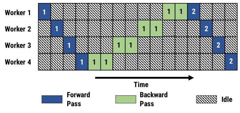
So it goes like this:

1. Worker 1 receives the original input (e.g. an image), processes it, and sends a feature map as input to Worker 2.
2. Worker 2 processes it further and sends it to Worker 3. Worker 3 does the same and sends it to Worker 4.
3. Worker 4 receives the feature maps, computes the final network output (e.g. an image class) and immediately starts computing the backward pass for its parameters (since it already has the final predictions and GT is available to it)
4. After computing the updates, it sends them to Worker 3, which in turn computes backpropagation for its portion of the model’s parameters. This gets repeated until Worker 1 finishes its updates.
5. After this the batch is processed, the optimization step is performed and the model is ready to process the next batch.

But hold on a minute, this is just sequential! It is not faster than training a model on a single device! And you’d be right:

However, since every device only stores a part of the model, it already certainly reduces the memory requirements of the GPUs. If your model takes ~40GB VRAM to train on a single batch, instead of buying a single A100 GPU for $7000, you could get away with e.g. 4 older GTX 1080 Ti 11Gb, which cost about $300 each (albeit, they would be quite a bit slower).

So it already has a use. But we can easily make it much better.

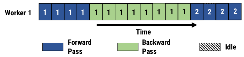
Filling the pipeline: take a look at Worker 1 in the first figure. Notice how it’s processed a single batch and then does nothing 75% of the time, until all the other workers are finished. Same for other workers.

If you count the total area of the blue and green cells per worker and compare it to the total time it takes for the whole pipeline to finish, you will see that our pipeline utilization is only 25%. Meaning, on average each worker spends 75% of the time doing nothing. This, in turn, means, that if we find something useful for the workers to do while they are waiting for other workers to finish, we can reduce idle time, increasing our efficiency (or “pipeline utilization”). If we manage to fill every cell in the chart, we will be looking at 100% pipeline utilization, 4x as many processed samples in the same amount of time, thus increasing our throughput by 4x.

pipeline_utilization = colored_area / total_area

So what should the workers do after they finished processing their data? What if they started to process the next data sample? And then the next? And then the next, until other workers after them finish and it’s time to do backpropagation? This is how it would look:

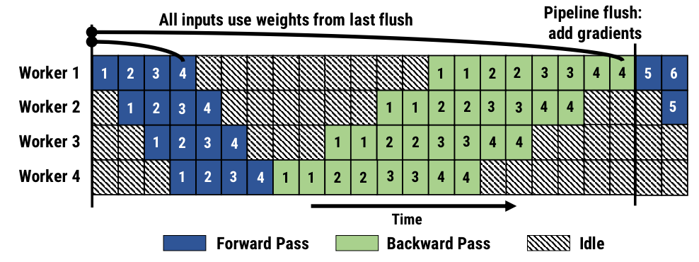
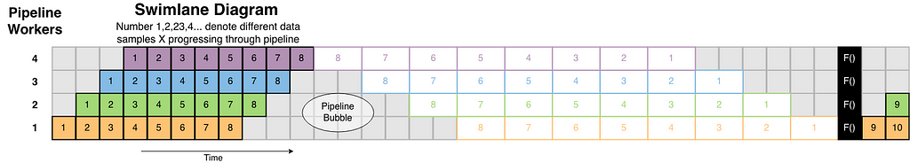
More formally, given k GPUs, a batch of N samples, we split our model into k sequential parts, each one stored on its own device, then we split the batch into m micro-batches of size (N/m), and feed them into our pipeline as illustrated in the picture. In practice m≥k. This is called All Forward All Backward (AFAB) parallelism, since all the workers will finish processing the forward pass before any of them start doing the backward pass.

Formal definition: how do we write this in terms of our aggregation function F and update function Δ?

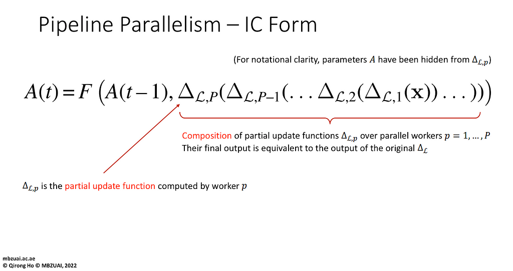
We split our Δ function into a composition (“nested calls”) of functions Δp, each responsible for computing the updates for a single device, taking as input the output of the previous Δp-1 function. This definition is flexible and doesn’t dictate to us how to feed micro-batches into the pipeline. Sequentially one-by-one? Yes. Filling out the pipeline like in the previous figure? Sure. Alternating between forward and backward passes for each device? Why not? All of these are plausible implementation details that do not break the backpropagation algorithm.

Memory usage. Our whole idea was to reduce memory usage, so let’s see how much memory each device needs. Let’s say that our model has A parameters that occupy O(A) memory; and each data sample needs O(1) memory in intermediate activations in the network (outputs of every layer), with the batch size of N taking — you guessed it — O(N) memory.

1. Each device stores a part of the model, so the overall memory occupied by the parameters would be O(A/k) — linearly decreasing with the number of devices being used (until you run out of layers). The more devices we have, the larger the model we can run, which is great.
2. The memory occupied by intermediate network outputs is also proportionally reduced by a factor of k — if I have 4 devices and a model with 16 layers, I only need to store activations of 4 layers on each device, which is also great! So more devices — larger models/input sizes (e.g. for images could allow using higher resolution).

What happens if we increase the batch size N? (reducing it is pointless as we want to keep the pipeline full, not empty) Let’s take a look:

Every device stores a part of every single sample’s intermediate activations, resulting in memory usage O(N/k) per device.

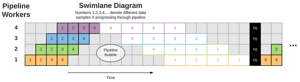
There are 3 idle parts in the diagram — the “startup”, the “cooldown” and the “bubble”. Either there is nothing to do, or the input is not ready yet — and the worker is idling — i.e. doing nothing. Right now utilization of this pipeline is at 57% (there are 48 colored cells and 84 total, 48/84=0.57). We want to improve it, so we naturally use a larger batch size. But how would the swimlane diagram look if we have 8 samples instead of 4?

This increases our pipeline utilization from 57% to 96/132=72%, but what about memory usage? Now each worker has to store activations for 8 samples instead of 4, so memory usage increased by a factor of 2x.

This limits the maximum batch size we can use during training, which is a bummer. If only there was a different way of organizing computations that will help us…

[Optional] Reduced memory usage — 1F1B: There is another, more efficient way to fill our pipeline with micro-batches:

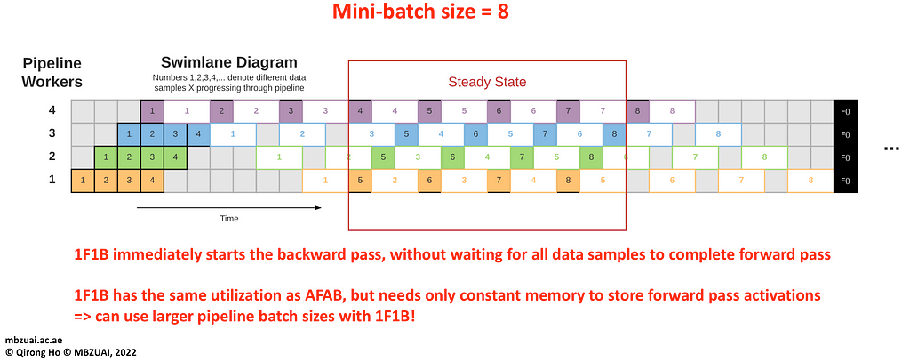
It’s called the “1 forward 1 backward” (1F1B) schedule — each worker will do a forward pass on a single micro-batch and then immediately do a backward pass on a different microbatch, and keep repeating — the only exception being the start and the finish of the pipeline.

This way every worker only has to keep O(1) intermediate activations in the memory, thus allowing us to increase the effective batch size almost indefinitely. Notice how in the diagram above each worker only has to keep information about 4 microbatches in its memory, even though our batch size can be infinitely large.

[Optional] Skip connections: What happens if you have skip connections in your network, especially long ones (e.g. in UNet)?

You can, of course, just copy the necessary data from device i to device i+1, then to device i+2, etc., until you reach the destination device j. This might seem inefficient, and it’s because it is.

Luckily, modern software libraries (e.g. GPipe and torchgpipe) solve this problem for you, allowing to bypass intermediate devices and copy the data directly from device i to device j like this. You can think of this mechanism as a “portal” between devices i and j, thus no more inefficient and unnecessary data copying.

Hybrid approaches

Can you use more than one type of parallelism when training your models? Yes, and you often should — to maximize the training speed and the hardware usage efficiency. But how do you do that?

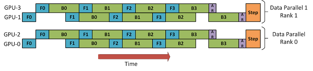
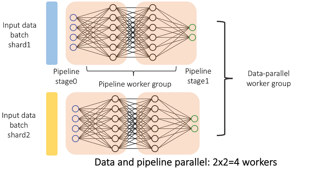
Perhaps the easiest way is to use Data Parallelism with anything else. Since it’s completely model-agnostic, it does not matter what you do to your model as long as the IC equation holds true (i.e. you don’t break backpropagation). So you can easily have e.g. 2 machines with 2GPUs in each, use Pipeline Parallelism across the GPUs to split your model into 2 sequential parts and assign one to each GPU in one machine; then clone this setup to the other machines, and use Data Parallelism across machines.

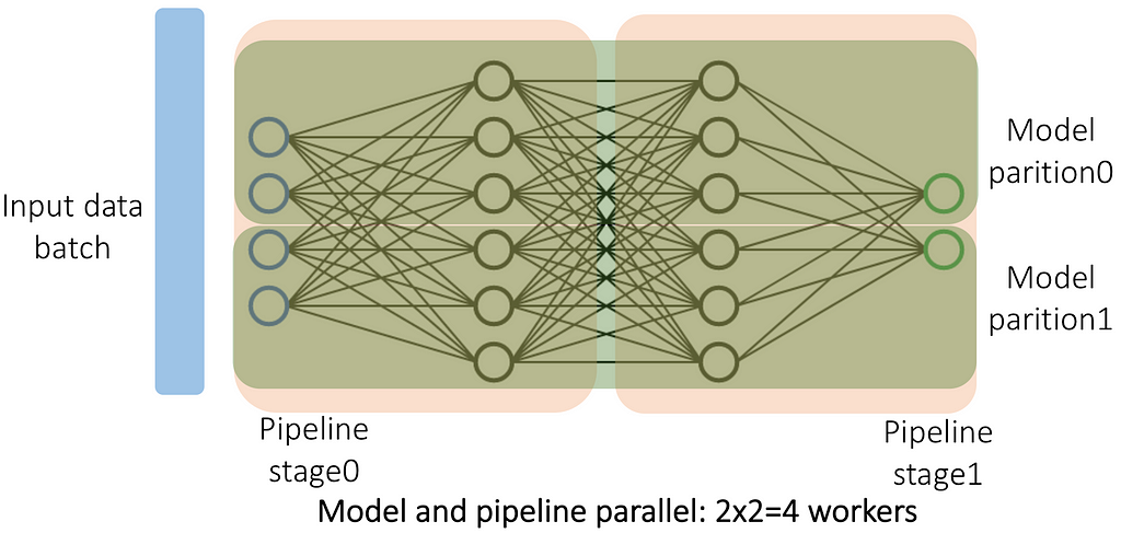
Okay, that seems simple enough, but can you combine Pipeline Parallelism and Model Parallelism? Yes, here is an illustration of how you can do it.

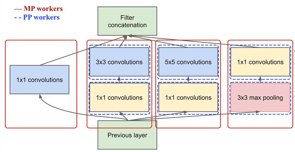
And it can be done the opposite way: first, we split the model into sequential chunks and then apply MP to each chunk individually, then the PP code does not need to know anything about deeper MP code.

Here is a summary of all pairs of combinations possible:

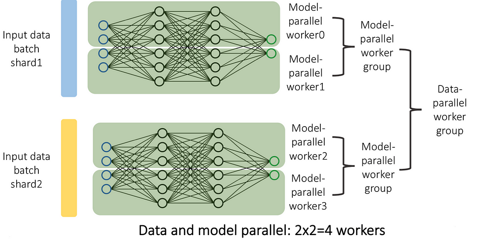
In practice, a typical arrangement in practice is as follows:

1. At the highest level, you have multiple Data Parallel clusters/sets of machines;
2. Each cluster/set of machines is running a Pipeline-Parallel version of your model, each pipeline stage taking a single machine;
3. Within each machine you can have multiple devices, and, as such, can further utilize Model Parallelism and/or Operator Parallelism to speed up computations and reduce memory usage.

Why would you use a hybrid approach? One reason is to utilize multi-level hardware — e.g. if you have multiple machines with multiple GPUs each, it makes more sense to use different types of parallelism together to more efficiently utilize your hardware (communicating between GPUs is different from communicating between machines, for example). E.g. having Model Parallelism across multiple machines will result in a huge communication overhead, while Data Parallelism and Model Parallelism would work just fine in such a setting.

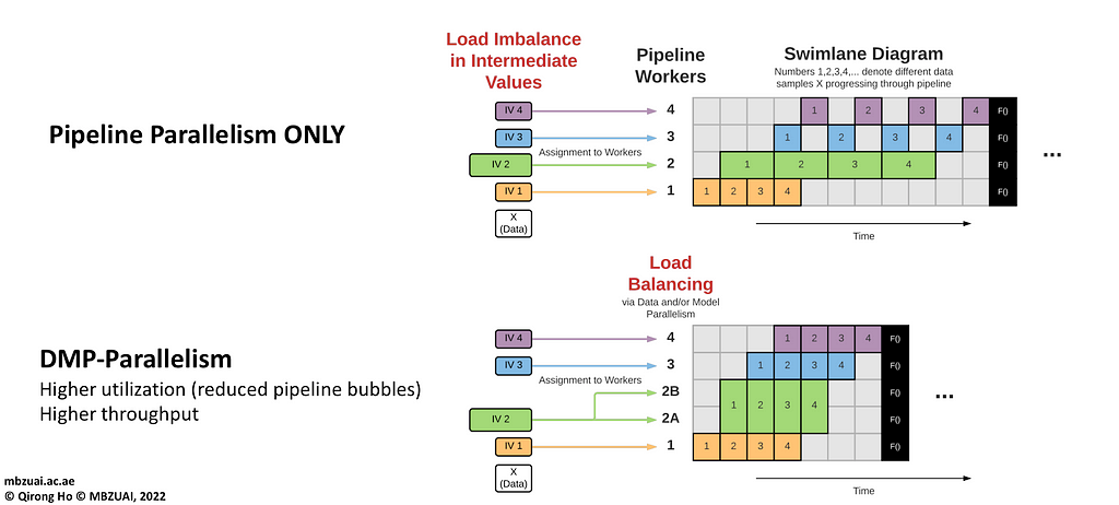
Another reason would be load-balancing: certain parts of your model could take more or less time/memory than others, and using a Hybrid parallelism approach would reduce your idle time at no additional costs, like in an example below:

When to use what

• Data Parallelism— if you don’t know what you’re doing, if your concern is convergence speed, your batch size right now is on the smaller side (e.g. < 64) and your model fits into a single GPU. Works fine on both single-machine and multi-machine configurations. Very easy to implement, typically already included in Deep Learning frameworks such as PyTorch and TensorFlow, a good place to start.
• Model Parallelism — if your model doesn’t fit into a single device, if your model has a lot of parallel branches/paths, or if you hate yourself and need high device utilization and memory efficiency. Not recommended to use across multiple machines due to high communication costs; you’ll likely have to implement it yourself for your particular model.
• Pipeline Parallelism — if your model doesn’t fit into a single device, but using Model Parallelism is too difficult. Works really well with sequential models like CNNs and Transformers, both across devices and across machines due to low communication cost between them. Not very hard to implement, a lot of existing software packages for Deep Learning models, might take you a few tries on how to split the model to balance the workload across devices.
• Hybrid Parallelism — if you’re training a really large model or a lot of large models. If you’re splitting your model across workers anyway, there is usually no reason not to throw Data Parallelism on top for quicker convergence.

Summary:

1. Compute Δ for subsets of samples in parallel — DataParallel
2. Compute Δ for subsets of parameters in parallel — ModelParalell
3. Split Δ into a composition of sequential steps — PipelineParallel
4. You can combine all three approaches in any way that seems practical

In the next part, we will cover metrics for Parallel and Distributed training, such as statistical efficiency, throughput, and goodput. We will see how to tell if our parallelized ML program is more efficient than our sequential single-worker program and look at common pitfalls when applying parallelization techniques.

---

An Introduction to Parallel and Distributed Training in Deep Learning was originally published in Better Programming on Medium, where people are continuing the conversation by highlighting and responding to this story.