Quality assurance is a goal that should be paramount for every professional software engineer. One of the components of this assurance is to make computer programs run smoothly and in acceptable latencies, i.e., write programs with low time complexities.
One widely known way of expressing the theoretical behavior of time or space complexity of computer algorithms is by applying asymptotic analysis.
Another metric, called cyclomatic complexity, was established by Thomas McCabe in his 1976 paper to determine a computer program’s stability and level of confidence.
But in day-to-day software development, a theoretical estimation of such complexities may not be accurate or feasible, especially when dealing with old legacy code bases.
This article shows how one can use the basics of asymptotic analysis to devise an experimental software setup to estimate time complexities.
A bit about fundamentals
Mathematically, we express the number of instructions of a program f as a function (sequence) f(n) > 0, where n (a natural number) denotes the problem size, e.g. the number of elements of a numeric array that will be manipulated by the software being analyzed.
To better understand how f behaves for increasing values of n, we classify the execution time function in question by asymptotically comparing f with another sequence g(n) > 0.
Using a more precise language, we ascertain the existence of a real-valued constant k > 0 and problem size m, such that f(n) ≤ kg(n), for all values of n > m. If we can find those numbers, we say that f(n) is of the order of g(n), or using asymptotic notation, f(n) = O(g(n)), where O(g(n)) is defined as:

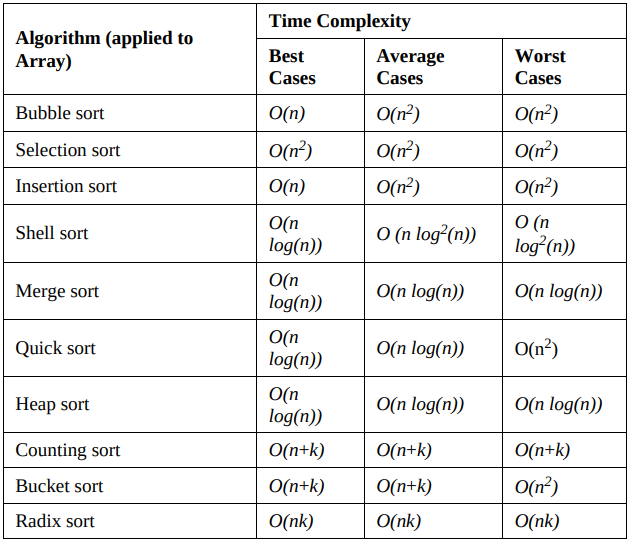
The following table summarizes the different time complexity theoretical behavior for the classical sorting algorithms of an array:

The proposed method
As I’ve mentioned previously, in some practical situations, the theoretical analysis of time complexities can be complicated by the state of the code implementation. But, using the concepts mentioned above, we can devise a way to estimate the time complexity by measuring the execution time of a program for increasingly bigger problems (values of n) and then comparing these time series with theoretical guessing functions.
To be more precise, suppose that my guess for an algorithm is quadratic, i.e., f(n) = O(n²). We are interested in the behavior of the values for the measured execution times, which will be represented by Tmeas(n). Using the asymptotic analysis formalism again, we are interested in studying the value of the bounding constant k, defined here as:

In the equation above:
- Tmeas(n): Corresponds to the measured execution time for a given problem size n, as mentioned earlier;
- Ttheory(n): Defined from the guessing “Big-O” bounding function g, it corresponds to the theoretical estimated value for the execution time. The constant α is here as a conversion factor, remembering that both functions f and g, by definition, give us the number of instructions to be made as a function of n, not the execution time. This constant also depends on the CPU architecture.
As n moves towards infinity, we can expect the following behaviors for k:
- Converges to zero: Our guess for g(n) is too low. Repeat with something bigger (e.g. g(n) = n³);
- Diverges to infinity: Our guess for g(n) is too high. Repeat with something smaller (e.g. g(n) = n log(n));
- Converges to a positive constant: Our guess is adequate. In other words, at least T_meas(n) approximates the theoretical complexity g(n) for as large n values as we tried.
These ideas now can be applied in a simple program to collect these time ratios and study their convergence. A simple prototype implementation in JavaScript could be like the one below:
// Optional. Just a generic way to type a function
type Callable<A = unknown[], B = unknown> = (
  ...args: A extends unknown[] ? A : [A]
) => B;

const problemSize = 1000;
const g: Callable<number, number> = n => n ** 2; // theoretical guess function
const timeRatios: number[] = [];
const m = 5; // from the O(g(n)) definition
const alpha = 1/127.372;  // Some suitable conversion constant that depends
                          // on the CPUs number of instructions per second.
let start = 0;

for (const n = m; i <= problemSize; n++) {
  try {
    start = performance.now();
    performanceSensitiveAlgorithm(n); // The code being analized
  } catch (error) {
    // Some appropriate error handling here.
  } finally {
    const measuredTime = performance.now() - start; // in ms
    const theoreticalTime = alpha * g(n) // now in ms
    timeRatios.push(theoreticalTime/measuredTime); // dimensionless ratios
  }
}
Proof of concept
To test this experimental methodology, I chose to implement a project in TypeScript called empirical-tc-ts which evaluates the time ratios for the classical implementation of the merge sort algorithm. I chose this algorithm because its asymptotic behavior is known to be g(n) = n log(n) (the logarithm here is of base 2) for both best and worst cases. So, this would be a good choice of guessing function to ascertain if the method is stable.
Concerning the conversion factor α, I’ve tested the execution in a laptop with an Intel Core i5-2500K processor, which can perform 83 MIPS (million instructions per second). Naturally, for simplification purposes, I’m not accounting here:
- How many clock cycles are necessary to perform one instruction;
- The effects of using multiple cores have different IPS values per clock per cycle.
So, assuming already that g is a rough estimation for the number of instructions of the algorithm in question, we can take the following definition of T_theory(n) with a grain of salt:

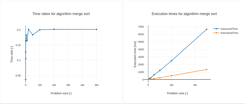
The first ratios were obtained for g(n) = n log(n). The results were:

For significant values of n, one can immediately verify the asymptotic behavior of the time ratios towards k = 0.2. For n = 5 million, the value for k is estimated to be 0.1988.
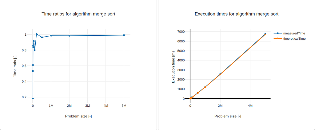
Tweaking more the guessing function, I now defined g(n) = 5n log(n). I’ve now obtained a more normalized result:

With the introduction of the scaling factor into g(n), the convergence was somewhat accelerated towards the unit, since the (pointwise) distance between the plots measuredTime and theoreticalTime was reduced. For n = 5 million, k = 0.9811.
Conclusion
As I mentioned before, the simplifications concerning CPU execution times and the very rough nature of asymptotic analysis make this method no substitute for more robust code profiling tools. However, with the above results, the developer could gain more immediate insight into the performance of some code sections just by understanding how asymptotic analysis works.
As for the to-do list, I believe that this method can be improved by integrating the following features:
- Improve the conversion factor calculation, as a function of the CPU specifications, by removing the simplifications that were made;
- Introduce repeatability and statistical analysis into the estimation of k. One can modify the implementation to run multiple batches for different sequences of problem sizes and extract the best value for k within a confidence interval from the resulting data.
Show me the code!
The project is published on GitHub and can be accessed from here.
The code was written using TypeScript, and the plots were generated using the NPM package nodeplotlib.
References
- Learning JavaScript Data Structures and Algorithms, 3rd edition, by Loiane Groner. It is available on Amazon.
- Wikipedia’s article on the merge sort algorithm: https://pt.wikipedia.org/wiki/Merge_sort
- Wikipedia’s article on processor’s IPS: https://en.wikipedia.org/wiki/Instructions_per_second
Determining Time Complexity of Algorithms Experimentally was originally published in Better Programming on Medium, where people are continuing the conversation by highlighting and responding to this story.