NBA Games Outcome Project — Model Development
Part 3 of 3

Hello! This is part three of a series where I build an end-to-end application that primarily aims to predict the game outcome between two chosen teams in a pool of 30 NBA professional teams. I am doing this series mainly to show the key aspects of what helped me create this project, as I learned a lot in the process, and I believe that knowledge should always be shared.
Objective
The main goal of this article is to feature the main concepts I used in the process of getting a working model and how you could apply them in your own projects. Here, we will try to train a machine-learning model that can beat the prediction model’s, NBA Oracle [1], performance. This project works with unseen data, and I took inspiration from it. The author says their project even beat the experts’ opinions, and the results are shown in the table below:

Setting up our reference metric
Initially, we want to see how a basic classification model performs on our ready-to-train data, and we are going to call it the baseline model. It will be our first reference, and we will aim to improve from it. Our r data from the 2021 and 2022 seasons has 1,200 game samples at the time of writing. So first, we will load our data with pandas and remove the existing columns to organize it. For example, the game date and season. We also allocate the column with the game’s outcome to the target vector and define it as y. The features column related to the matrix will be defined as x.
From now on, we will heavily use the library scikit-learn, which is the most popular library for machine learning in Python. With this tool in our hands, we can now train data from test data separately and train our baseline model, a Logistic Regression. We only need to adjust the max_iter parameter to a large number so it can converge on our data. We can visualize our results with a nice ConfusionMatrixDisplay method from sklearn; this will show our confusion matrix, as seen below. You have to plug in your model, the test features, and the test target.

With the train and test split method from scikit-learn, we get a nice accuracy of 72.6% on the test set! Cross-validation is a nice way to test the models’ predictions as it separates the data in batches and train-tests multiple times, where each fraction of the data is used as training and also as a test eventually. You can get more information from the sklearn page if you want to know the details.
Using cross-validation scores with five batches, we get a superior accuracy of 74.3%! For me, this is a lesson of why quality data matters and why it is worth investing the time to get to it, as we already surpassed the reference we had to beat and could go home from here — just kidding. Because we have our new reference now, let’s see what we can do to improve it!
Developing new models

We are going to try four models, all through Scikit-learn. The first will be Logistic Regression; this is good to analyze first because of its simplicity and efficiency. Then we go with Support Vector Machines (SVMs), which are good for high-dimension data because of their kernel and our dataset’s hundreds of features.
Finally, we will try the ensemble models of random forest and gradient boosting classifier, which require more parameters, are built on top of decision trees, and allow us to capture complex patterns within the data that would be impossible otherwise.
Initially, the data for training the models will be the same as we used for the baseline model. To maintain the code cleaner and reusability, we create a Python class, ModelParams, to hold the range of parameters for each model. For example, we custom-made it to have a set of penalty parameters for logistic regression, namely l1, l2, and elasticnet (the mix of l1 and l2).
This class will also have the data scaler attributes, the Standard Scaler for the linear models, and the MinMax Scaler for the ensembles. The ensemble models work without the need to scale data because of how the decision trees choose the features that cause the most impact on the target variable. So, when calling this class, we instantiate a pipeline object with the model we want — with or without a scaler — and all the set of parameters associated with this model. It will also have a method that allows us to visualize the model, scaler, and parameter ranges after instantiation.
We create a second class, ModelDevelopment, that can take in the pipeline we made previously, as well as the features X and target y data, to be first instantiated. Two methods give the training functionality of the class: one is used to train the model against all the sets of tuning parameters, named grid_search, and the other is used to train against random parameters within the passed group. We named this random_search. It also has methods we can use to analyze the metrics and AUC ROC curve of a method after training.
The grid_search method uses the GridSearchCV from scikit-learn. It’s responsible for training our model n*folders times (brute force). n is the combined result when using all the features of the set we passed, and the folders are the cross-validation split. It also has the option to choose the scoring metric that goes into the train. The method returns the best model, best parameters, and best score for this best model. It has the attributes of all scores, too, if we wish to access it. We will use this method to find the optimal parameters of the linear models, as they have fewer parameters to combine and are faster to train when compared with more complex models.
The random_search method uses the RandomizedSearchCV from scikit-learn. It does everything grid_search does, with the exception that it will train our model z*folders times. z is a subset of random tuning parameters of the n set. We will train our ensemble models as we can set the number of training steps. The drawback of many parameters is that we have to tune them, and the model complexity increases the training time compared with the linear models.
As for validation analysis, the class has a method named model_metric to see the scores related to accuracy, precision, recall, f1, and auc. It also has a method that plots the auc roc curve, and it is named roc_curve. A third method is used to plot the confusion matrix of the model, and it’s named plot_confusion_matrix. After using the training functions, these methods will take in the optimal parameters as class attributes of the chosen model, so they don’t need arguments passed.
Now, we plug everything in and see what parameters we get for each model. Using the x and y train and test, the results are around 72% — 76% for the gradient boosting classifier model.
As we can see, they are close to the baseline model, which was 72.6%. It implies that we did our best to tune the models, but it only improves our accuracy slightly. What can we do to try and improve this? The answer is the classic: let’s play with our data!
Improving data quality with feature selection

Our training data began with 269 features, which is a lot. We will narrow it so only the features that cause the higher variance in our model are part of the final training data.
We will perform feature selection in three ways: First, through exhaustive feature selection using the SequentialFeatureSelector from sklearn. Then through analytical selection using SHAP, a Python library that is very popular in visualizing features’ importance and how they impact the model. Finally, we will use the Principal Component Analysis (PCA) technique to select the best features for the model.
The first method trains the model with one subset of features at a time. It goes through each feature, and we can choose if it moves from one feature to all features (direction = forward)… or if it starts from all features and ends at one feature (direction = backward). Hence the exhaustive concept. We must pass the model, direction, number of features, and metric score as arguments to the SequentialFeatureSelector method. Below we can see the code snippet that’s been customized for this task:
from sklearn.feature_selection import SequentialFeatureSelector
from time import time
import os

def select_nBest_features(model, n_features):
    """ Info:
     Choose a model and a number of features to select the best features among this number, saving the results in a csv file,
     plots the top n_best_features and returns a dataframe with the feature importance.
     As the method dont return the importances, just the most important features, we need to get to that after the selection.
      -----------------------------------------------------------------------------------------------------------------
       Input:
        model: The model to be used.
        n_features: The number of best features to select
        -----------------------------------------------------------------------------------------------------------------
            Output:
                Best features for the chosen model.

            """
    #verifies if the model is saved already to proceed with the selection
    if not os.path.isfile(f'best_features/{model[-1].__class__.__name__}_{n_features}.csv'): # model[-1] is the model itself in the pipeline
        start = time()
        sfs = SequentialFeatureSelector(model[-1], n_features_to_select=n_features, direction='backward', scoring='accuracy', cv=5, n_jobs=-1)
        sfs.fit(X, y)
        end = time()
        print(f"Features selected by forward sequential selection: {X.columns[sfs.get_support()]}") #feature names for the best features
        print(f'Minutes elapsed: {round((end - start)/60)}') #time in minutes
        #saving the best features to csv
        pd.Series(X.columns[sfs.get_support()]).to_csv(f'best_features/{model[-1]}_{n_features}.csv', index=False)
    else:
        print(f'Best {n_features} features for {model[-1].__class__.__name__} already saved.')

    #loading the best features for plotting
    return pd.read_csv(f'best_features/{model[-1].__class__.__name__}_{n_features}.csv', header=None)
The second method is about the SHAP, so we can get the visuals based on JavaScript. Being able to see the features’ contributions will help us see how much each explains the model’s variance.
Note: we need to pass the data scaled for the SHAP because we can’t pass the pipelined model. We can only use the model contained in the last step of the previous pipe (scaler + model). For example, if we want to see what the top 10 most impactful features of the random forest model are, we could do something like this:
# Create SHAP explainer
explainer = shap.TreeExplainer(RF[-1], X_scaled, seed=42)
shap_values = explainer.shap_values(X_scaled)

plt.figure(figsize=(10, 10))
shap.summary_plot(shap_values, X_scaled, max_display=10, plot_type='bar')
plt.tight_layout()
plt.show()
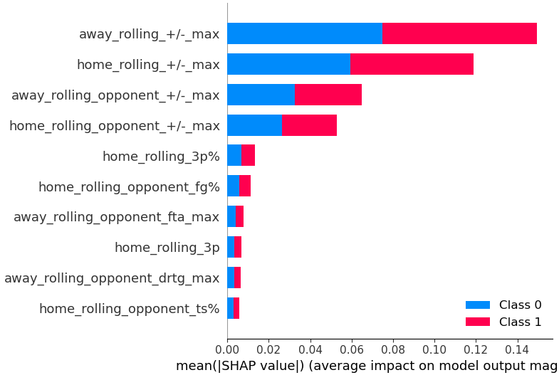
This way, we can get insights into how many features we choose. In this example, we could try only the first four features to train our ensembled models.
The last method is the use of PCA to get the dimensionality reduction. So basically, we want PCA to transform n data features into m principal components, where m<n. The components are orthogonal vectors that approximate the data with least squares, extracting the most important aspects underlining. For this, we must pass our data scaled first by subtracting the mean and getting data points around the unit variance. To understand the intuition behind PCA, I recommend this link.
We will get a sense of how much of our 269 features are explained with the principal components by studying the graph below:

Nice. We can see that the first 100 principal components can explain around 95% of our data variation. What we can do now is transform our data features into 100 principal components and see if we can increase the accuracy and other metrics given by the sklearn method using classification_report.
from sklearn.decomposition import PCA

def pca_metrics(model, X_train=X_train_scaled, X_test=X_test_scaled, y_train=y_train, y_test=y_test, n_components=0.95):
    """ Info:
     This function takes a model and returns the metrics reports of the model with the PCA.
      -----------------------------------------------------------------------------------------------------------------
       Input:
        model: The model to be used.
        X_train: The training set.
        X_test: The testing set.
        y_train: The training target.
        y_test: The testing target.
        n_components: The number of components to be used in the PCA.
        -----------------------------------------------------------------------------------------------------------------
        Output:
         classification_report: The classification report of the model with the PCA.
        """
    pca = PCA(n_components=n_components)
    X_train_pca = pca.fit_transform(X_train)
    X_test_pca = pca.transform(X_test)
    model.fit(X_train_pca, y_train)
    y_pred = model.predict(X_test_pca)
    #get the number of components
    n_components = pca.n_components_

    return classification_report(y_test, y_pred), n_components
# using 100 principal components to train and test our models
models = [lr, svm, rf, gbc]

for model in models:
    print('{}n'.format(model[1]), pca_metrics(model, n_components=100)[0])
    print('Principal components used: {}n'.format(pca_metrics(model, n_components=100)[1]))
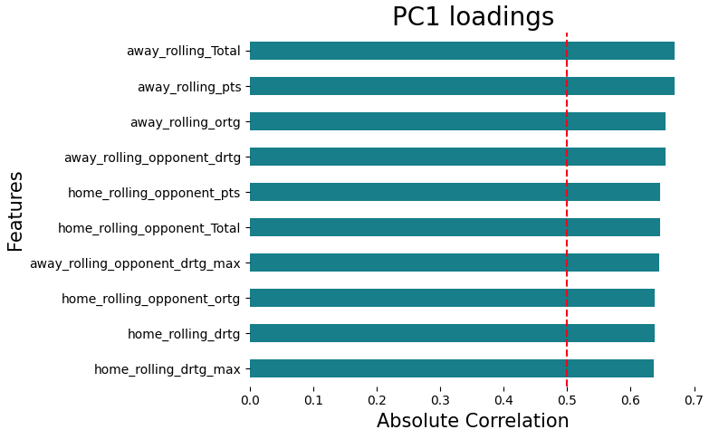
Still, with PCA, we could also use it to select the best features without transformation. For example, we could select the top 10 features that are most correlated with the first principal component. You can see how this works in the following code:
plt.figure(figsize=(10, 20))

loadings = pd.DataFrame(
    data=pca.components_.T * np.sqrt(pca.explained_variance_), #type: ignore
    columns=[f'PC{i}' for i in range(1, len(X_train.columns) + 1)], #type: ignore
    index=X_train.columns #type: ignore
)
loadings['PC1'] = abs(loadings['PC1'])
#picking the 100 best featues accordnly to PCA 1
pca_best_features = loadings['PC1'].sort_values(ascending=False).head(100)

pca_best_features[::-1].plot(kind='barh', color='#087E8B')
plt.title('PC1 loadings', size=20)
plt.ylabel('Features', size=15)
plt.xlabel('Absolute Correlation', size=15)

#drawing a line at 0.5
plt.axvline(x=0.5, color='red', linestyle='--')

pca_best_features.head(10)
Well, let’s recap what we did:
- Trained and tested the models against data with a specific set of features
- Selected the best hyperparameters
- Selected the best data features with the models with their hyperparameters from before
The next phase involves repeating these steps. We can keep iterating until we are satisfied with our results.
Results
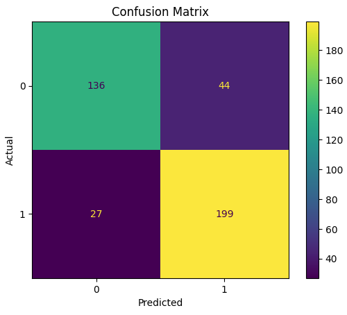
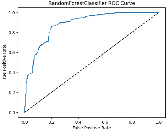
By doing this process, we find out that the best model was the random forest, with about 82.5% accuracy and 81.8% AUC. It was trained on data with the 50 best features selected by the exhaust feature selection technique, so that’s the one we are going to use. Some of the model stats follow:
{'randomforestclassifier__n_estimators': 1000,
 'randomforestclassifier__min_weight_fraction_leaf': 0.0,
 'randomforestclassifier__min_samples_split': 10,
 'randomforestclassifier__min_samples_leaf': 2,
 'randomforestclassifier__min_impurity_decrease': 0.0,
 'randomforestclassifier__max_leaf_nodes': 31,
 'randomforestclassifier__max_features': 'sqrt',
 'randomforestclassifier__max_depth': 7,
 'randomforestclassifier__criterion': 'entropy'}
Final Thoughts
I want to wrap it up by stating that we should not pursue the perfect model. As data changes, the metrics will also change, and this is relevant when we talk about basketball games — where the weaker team could win against all odds. There will always be a way to improve the ML pipeline, which will mostly happen on the data quality. I presented some ways you could use to get a proper and decent model running, so try some of these depending on your project’s needs.
On my GitHub, this analysis’s notebooks are documented, organized, and, hopefully, educational! The final step will be a wrap-up of everything and a chance to see this project deployed in the cloud. And yes, the data will be fed automatically!
Want to Connect?

If you want, please contact me on my LinkedIn for any feedback or questions.
I will be happy to answer.
References
[1] M. Beckler, H. Wang, M. Papamichael. ‘NBA Oracle,’ Pittsburgh, 2013.
NBA Games Outcome Project — Model Development was originally published in Better Programming on Medium, where people are continuing the conversation by highlighting and responding to this story.